hypothesis test critical region

User Preferences

Content preview.

Arcu felis bibendum ut tristique et egestas quis:

• Ut enim ad minim veniam, quis nostrud exercitation ullamco laboris
• Duis aute irure dolor in reprehenderit in voluptate
• Excepteur sint occaecat cupidatat non proident

Keyboard Shortcuts

S.3.1 hypothesis testing (critical value approach).

The critical value approach involves determining "likely" or "unlikely" by determining whether or not the observed test statistic is more extreme than would be expected if the null hypothesis were true. That is, it entails comparing the observed test statistic to some cutoff value, called the " critical value ." If the test statistic is more extreme than the critical value, then the null hypothesis is rejected in favor of the alternative hypothesis. If the test statistic is not as extreme as the critical value, then the null hypothesis is not rejected.

Specifically, the four steps involved in using the critical value approach to conducting any hypothesis test are:

• Specify the null and alternative hypotheses.
• Using the sample data and assuming the null hypothesis is true, calculate the value of the test statistic. To conduct the hypothesis test for the population mean μ , we use the t -statistic \(t^*=\frac{\bar{x}-\mu}{s/\sqrt{n}}\) which follows a t -distribution with n - 1 degrees of freedom.
• Determine the critical value by finding the value of the known distribution of the test statistic such that the probability of making a Type I error — which is denoted \(\alpha\) (greek letter "alpha") and is called the " significance level of the test " — is small (typically 0.01, 0.05, or 0.10).
• Compare the test statistic to the critical value. If the test statistic is more extreme in the direction of the alternative than the critical value, reject the null hypothesis in favor of the alternative hypothesis. If the test statistic is less extreme than the critical value, do not reject the null hypothesis.

Example S.3.1.1

Mean gpa section  .

In our example concerning the mean grade point average, suppose we take a random sample of n = 15 students majoring in mathematics. Since n = 15, our test statistic t * has n - 1 = 14 degrees of freedom. Also, suppose we set our significance level α at 0.05 so that we have only a 5% chance of making a Type I error.

Right-Tailed

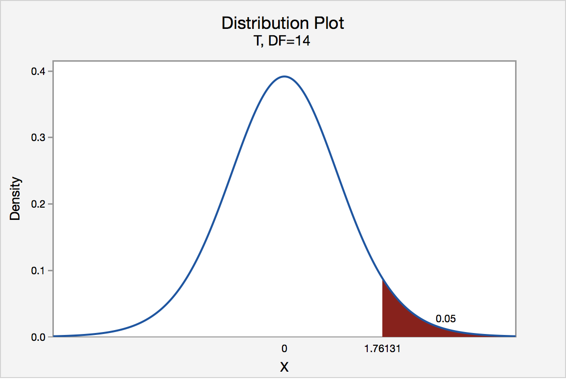
The critical value for conducting the right-tailed test H 0 : μ = 3 versus H A : μ > 3 is the t -value, denoted t \(\alpha\) , n - 1 , such that the probability to the right of it is \(\alpha\). It can be shown using either statistical software or a t -table that the critical value t 0.05,14 is 1.7613. That is, we would reject the null hypothesis H 0 : μ = 3 in favor of the alternative hypothesis H A : μ > 3 if the test statistic t * is greater than 1.7613. Visually, the rejection region is shaded red in the graph.

Left-Tailed

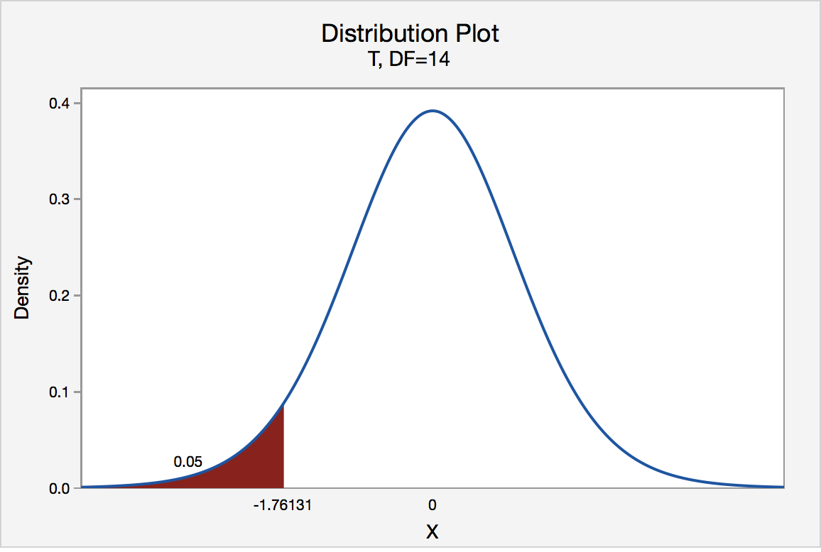
The critical value for conducting the left-tailed test H 0 : μ = 3 versus H A : μ < 3 is the t -value, denoted -t ( \(\alpha\) , n - 1) , such that the probability to the left of it is \(\alpha\). It can be shown using either statistical software or a t -table that the critical value -t 0.05,14 is -1.7613. That is, we would reject the null hypothesis H 0 : μ = 3 in favor of the alternative hypothesis H A : μ < 3 if the test statistic t * is less than -1.7613. Visually, the rejection region is shaded red in the graph.

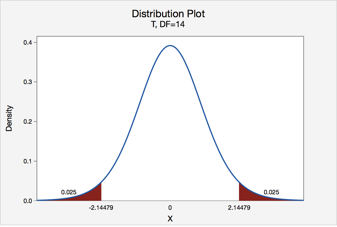
There are two critical values for the two-tailed test H 0 : μ = 3 versus H A : μ ≠ 3 — one for the left-tail denoted -t ( \(\alpha\) / 2, n - 1) and one for the right-tail denoted t ( \(\alpha\) / 2, n - 1) . The value - t ( \(\alpha\) /2, n - 1) is the t -value such that the probability to the left of it is \(\alpha\)/2, and the value t ( \(\alpha\) /2, n - 1) is the t -value such that the probability to the right of it is \(\alpha\)/2. It can be shown using either statistical software or a t -table that the critical value -t 0.025,14 is -2.1448 and the critical value t 0.025,14 is 2.1448. That is, we would reject the null hypothesis H 0 : μ = 3 in favor of the alternative hypothesis H A : μ ≠ 3 if the test statistic t * is less than -2.1448 or greater than 2.1448. Visually, the rejection region is shaded red in the graph.

Critical Region and Confidence Interval

Contents Toggle Main Menu 1 Confidence Interval 2 Significance Levels 3 Critical Region 4 Critical Values 5 Constructing a Confidence Interval 5.1 Binomial Distribution 5.2 Normal Distribution 5.3 Student $t$-distribution 6 Video Examples

Confidence Interval

A confidence interval , also known as the acceptance region, is a set of values for the test statistic for which the null hypothesis is accepted. i.e. if the observed test statistic is in the confidence interval then we accept the null hypothesis and reject the alternative hypothesis .

Significance Levels

Confidence intervals can be calculated at different significance levels . We use $\alpha$ to denote the level of significance and perform a hypothesis test with a $100(1- \alpha)$% confidence interval.

Confidence intervals are usually calculated at $5$% or $1$% significance levels, for which $\alpha = 0.05$ and $\alpha = 0.01$ respectively. Note that a $95$% confidence interval does not mean there is a $95$% chance that the true value being estimated is in the calculated interval. Rather, given a population, there is a $95$% chance that choosing a random sample from this population results in a confidence interval which contains the true value being estimated.

Critical Region

A critical region , also known as the rejection region, is a set of values for the test statistic for which the null hypothesis is rejected. i.e. if the observed test statistic is in the critical region then we reject the null hypothesis and accept the alternative hypothesis.

Critical Values

The critical value at a certain significance level can be thought of as a cut-off point. If a test statistic on one side of the critical value results in accepting the null hypothesis, a test statistic on the other side will result in rejecting the null hypothesis.

Constructing a Confidence Interval

Binomial distribution.

Usually, the easiest way to perform a hypothesis test with the binomial distribution is to use the $p$-value and see whether it is larger or smaller than $\alpha$, the significance level used.

Sometimes, if we have observed a large number of Bernoulli Trials, we can use the observed probability of success $\hat{p}$, based entirely on the data obtained, to approximate the distribution of error using the normal distribution. We do this using the formula \[\hat{p} \pm z_{1-\frac{\alpha}{2} } \sqrt{ \frac{1}{n} \hat{p} (1-\hat {p})}\] where $\hat{p}$ is the estimated probability of success, $z_{1- \frac{\alpha}{2} }$ is obtained from the normal distribution tables , $\alpha$ is the significance level and $n$ is the sample size.

Worked Example

A coin is tossed $1050$ times and lands on heads $500$ times. Construct a $90$% confidence interval for the probability $p$ of getting a head.

Here the observed probability of success $\hat{p} = \dfrac{500}{1050}$, $n=1050$ and $\alpha = 0.1$ so $z_{1-\frac{\alpha}{2} } = z_{0.95} = 1.645$. This is because $\Phi^{-1} (0.95) = 1.645$ .

So the confidence interval will be between $\hat{p} + z_{1-\frac{\alpha}{2} } \sqrt{ \frac{1}{n} \hat{p} (1-\hat {p})} \text{ and } \hat{p} - z_{1-\frac{\alpha}{2} } \sqrt{ \frac{1}{n} \hat{p} (1-\hat {p})} . $ By substituting into these expressions, we find that the confidence interval is between \begin{align} &\dfrac{500}{1050} + 1.645 \sqrt{ \frac{1}{1050} \times \dfrac{500}{1050} \times \left(1- \dfrac{500}{1050}\right) }\\ \text{ and } &\dfrac{500}{1050} - 1.645 \sqrt{ \frac{1}{1050} \times \dfrac{500}{1050} \times \left(1- \dfrac{500}{1050}\right) }\\\\ &=0.47619 + (1.645 \times \sqrt{0.00024} ) \text{ and } 0.47619 - (1.645 \times \sqrt{0.00024} ) \\ &=0.50155 \text{ and } 0.45084 . \end{align} So the confidence interval is $(0.45084, 0.50155)$.

Normal Distribution

We can use either the $z$-score or the sample mean $\bar{x}$ as the test statistic. If the $z$-score is used then reading straight from the tables gives the critical values.

For example, the critical values for a $5$% significance test are:

To obtain a confidence interval for the mean, use the following procedure:

For a two-tailed test with a $5$% significance level we need to consider \begin{align} 0.95 &= \mathrm{P}[-k< Z < k] \\ &= \mathrm{P}\left[-k<\dfrac{\bar{X}-\mu}{\frac{\sigma}{\sqrt{n} } } \mu+1.96\frac{\sigma}{\sqrt{n} }. \]

Student $t$-distribution

Given the number of degrees of freedom $v$ and the significance level $\alpha$, the critical values can be obtained from the tables. Critical regions can then be computed from these.

If we are performing a hypothesis test at a $1$% significance level with $15$ degrees of freedom using the Student $t$-distribution then there are three cases, depending on the alternative hypothesis.

If we are performing a two-tailed test, the critical values are $\pm2.9467$ so the confidence interval is $-2.9467 \leq t \leq 2.9467$ where $t$ is the test statistic. The critical regions will be $t< -2.9467$ and $t>2.9467$.

If we are performing a one-tailed test, the critical value is $2.6025$:

Video Examples

In this video, Daniel Organisciak calculates a one-tailed confidence interval for the normal distribution.

In this video Daniel Organisciak calculates a two-tailed confidence interval for the normal distribution.

All Subjects

Theoretical Statistics

Study guides for every class, that actually explain what's on your next test, critical region, from class:.

The critical region is a set of values for a test statistic that leads to the rejection of the null hypothesis in statistical hypothesis testing. This region is determined based on the significance level, often denoted as alpha (\(\alpha\)), which defines the probability of making a Type I error. The critical region plays a vital role in determining whether the observed data provide sufficient evidence against the null hypothesis, guiding decision-making in statistical inference.

congrats on reading the definition of Critical Region . now let's actually learn it.

5 Must Know Facts For Your Next Test

• The critical region corresponds to the extreme values of a test statistic that are unlikely under the null hypothesis, usually determined by the significance level chosen.
• In a two-tailed test, the critical region is split between both tails of the distribution, while in a one-tailed test, it is located entirely in one tail.
• Common distributions used to determine critical regions include the normal distribution, t-distribution, and chi-squared distribution.
• The size of the critical region directly affects the power of the test; a larger critical region increases the chance of rejecting the null hypothesis but also raises the risk of a Type I error.
• Critical values marking the boundaries of the critical region are calculated based on the chosen significance level and the distribution of the test statistic.

Review Questions

• The significance level determines how extreme the values must be for the test statistic to fall into the critical region and thus lead to rejection of the null hypothesis. For example, with a significance level of \(\alpha = 0.05\), the critical region would typically encompass 5% of the probability distribution's tails. This means if your test statistic falls within this area, you have sufficient evidence to reject the null hypothesis.
• In a one-tailed test, the critical region is located entirely in one tail of the distribution, indicating that we are only testing for an effect in one direction. In contrast, a two-tailed test has critical regions in both tails, which allows for detection of effects in both directions. This distinction affects how we interpret our results; a one-tailed test can be more powerful for detecting directional effects but may miss out on discovering effects in the opposite direction.
• As sample size increases, the standard error decreases, resulting in a more concentrated test statistic distribution around its mean. This change can lead to smaller critical values for a given significance level, making it easier to reject the null hypothesis even with minor effects. Therefore, larger samples can enhance power by reducing variability and increasing confidence in statistical decisions, which can impact how researchers interpret their results regarding significant findings.

Related terms

Null Hypothesis : A statement that there is no effect or no difference, serving as the default assumption to be tested against.

The error made when the null hypothesis is rejected when it is actually true, leading to a false positive conclusion.

Significance Level : The threshold probability (often \(\alpha = 0.05\)) set by the researcher for deciding whether to reject the null hypothesis.

" Critical Region " also found in:

Subjects ( 5 ).

• Data Science Statistics
• Engineering Probability
• Honors Statistics
• Intro to Statistics
• Statistical Methods for Data Science

© 2024 Fiveable Inc. All rights reserved.

Ap® and sat® are trademarks registered by the college board, which is not affiliated with, and does not endorse this website..

• Biochemistry
• Bioengineering
• Cancer Research
• Developmental Biology
• Engineering
• Environment
• Immunology and Infection
• Neuroscience
• JoVE Journal
• JoVE Encyclopedia of Experiments
• JoVE Chrome Extension
• Environmental Sciences
• Pharmacology
• JoVE Science Education
• JoVE Lab Manual
• JoVE Business
• Faculty Resource Center
• For Libraries
• For Higher Education Courses
• For High Schools
• High Schools
• JoVE High schools
• Videos Mapped to Your Course

Critical Region, Critical Values and Significance Level

Previous video 9.2: null and alternative hypotheses, next video 9.4: p -value, 9,979 views.

The critical region, critical value, and significance level are interdependent concepts crucial in hypothesis testing.

In hypothesis testing, a sample statistic is converted to a test statistic using z , t , or chi-square distribution. A critical region is an area under the curve in  probability distributions demarcated by the critical value. When the test statistic falls in this region, it suggests that the null hypothesis must be rejected. As this region contains all those values of the test statistic (calculated using the sample data) that suggest rejecting the null hypothesis, it is also known as the rejection region or region of rejection. The critical region may fall at the right, left, or both tails of the distribution based on the direction indicated in the alternative hypothesis and the calculated critical value.

A critical value is calculated using the z , t, or chi-square distribution table at a specific significance level. It is a fixed value for the given sample size and the significance level. The critical value creates a demarcation between all those values that suggest rejection of the null hypothesis and all those other values that indicate the opposite. A critical value is  based on a pre-decided significance level.

A significance level or level of significance or statistical significance is defined as the probability that the calculated test statistic will fall in the critical region. In other words, it is a statistical measure that indicates that the evidence for rejecting a true null hypothesis is strong enough. The significance level is indicated by α, and it is commonly 0.05 or 0.01.