our Stories
October 21, 2021

The Clean Water Case of the Century

The nation's highest court sided with clean water advocates in a decades-long legal dispute involving a wastewater treatment plant, its pollution discharges, and a partially dead coral reef in Hawaiʻi.
“This decision is a huge victory for clean water,” said David Henkin , the Earthjustice attorney who argued the case before the U.S. Supreme Court.
Our Clients Hawaiʻi Wildlife Fund, Sierra Club-Maui Group, Surfrider Foundation, West Maui Preservation Association Read the Supreme Court Decision
In 2020, the U.S. Supreme Court issued its decision solidifying the Clean Water Act’s place as one of the nation’s most effective environmental laws.
The following year, in the first application of the Supreme Court's test, the Hawai‘i district court reaffirmed protections for the nation's waters.
What started as a local water pollution case could have had disastrous repercussions for clean water across the United States.
What did the U.S. Supreme Court decide?
The U.S. Supreme Court's decision leaves in place vital protections for the nation’s oceans, rivers, and lakes.
The court found that point source discharges to navigable waters through groundwater are regulated under the Clean Water Act. In its decision on County of Maui v. Hawai ʻ i Wildlife Fund , the court held that the Clean Water Act “require[s] a permit if the addition of the pollutants through groundwater is the functional equivalent of a direct discharge from the point source into navigable waters.”
In other words, the Clean Water Act prohibits unpermitted discharge of pollution “into navigable waters, or when the discharge reaches the same result through roughly similar means.”
In doing so, the Court rejected the Trump administration’s polluter-friendly position in the clearest of terms: “We do not see how Congress could have intended to create such a large and obvious loophole in one of the key regulatory innovations of the Clean Water Act.”
The opinion was written by Justice Breyer with a vote of 6-3; with Chief Justice Roberts joining the opinion, along with Ginsburg, Sotomayor, Kagan, and Kavanaugh. (Learn about what happens next with this case, following the Supreme Court's decision.)
Abigail Dillen, President of Earthjustice, explains what happened and what the ruling means:
It’s stunning to think how close we came to a world where industries could just point their pipes straight down into groundwater to dispense of their pollution indirectly into clean water without repercussion. — Abbie Dillen (@AbbieDillen) April 23, 2020
What happened during oral arguments at the U.S. Supreme Court?
Earthjustice attorney David Henkin presented oral arguments in November, before the nine Justices of the U.S. Supreme Court in County of Maui v. Hawaiʻi Wildlife Fund
The Justices posed tough questions to both sides. (Read the transcript.) A summary of the hearing:
- The County’s interpretation of the Clean Water Act is that a “point source” (such as a pipe) must be the thing that delivers pollution for it to be regulated. That, once in groundwater or not straight from the “point source,” the Clean Water Act does not regulate that discharge.
- A few Justices feared the County’s position would create a roadmap for polluters to evade regulation. Justice Breyer asked: What if we end the pipe five feet from the ocean?
- Justice Kagan doubled down, saying nobody would get a permit if they could cut the pipe a few feet short.
- But the Justices also asked Earthjustice attorney Henkin: What should be a definition for a limit to what is regulated? Would this interpretation mean homeowners' septic tanks that leach through groundwater to a river need to get permits under the Clean Water Act (or face stiff fines).
- Henkin explained that pollution that is “traceable” and a “proximate cause” would be regulated and that for three decades, U.S. EPA had gone with that interpretation without millions of homeowners on the hook for pollution from their septic tanks. ( More on the back and forth over the Justice’s questions on limits. )
- The County also deflected responsibility back to the states, saying state groundwater permitting, grant programs, etc., are sufficient to regulate that flows from a point source (such as Maui County’s wastewater wells) through groundwater and to a protected body of water.
- Justice Sotomayor interjected that that’s a problem because it presumes the state will regulate that pollution. Justice Kagan also stated that this case isn’t about relying on state backstops.
- The attorney for the U.S. Government made an analogy about spiking a punch with whiskey . Henkin deftly turned it back around.
The attorney for the U.S. Government made an analogy about spiking a punch with whiskey. Henkin deftly turned it back around. @Earthjustice ’s Sam Sankar explains here. pic.twitter.com/XZrQIjAQM3 — Earthjustice (@Earthjustice) November 6, 2019
- Justices generally seemed to reject the County's extreme position that only pollution direct from a point source is regulated, so pollution sprayed through air or that travels over ground would also be free of Clean Water Act regs. But they seemed unsure how far to go.
- At the end, Justice Sotomayor brought it home asking: What current regulations exist that stop the county from polluting the ocean? It’s definitely happening, and Maui County says the Clean Water Act shouldn't stop them — so are they just going to get away with it? What is being done to stop this?
. @Earthjustice attorney David Henkin gives his final thoughts on defending America's clean water in front of the Supreme Court, likely the biggest day of his career. #CleanWaterActIntact pic.twitter.com/b6k9I8nflc — Earthjustice (@Earthjustice) November 6, 2019
What’s County of Maui v. Hawai‘i Wildlife Fund about?
At its most basic level, this case was about whether a wastewater treatment facility in Maui is violating the Clean Water Act by polluting the ocean indirectly through groundwater.
Since the 1980s, Maui’s Lahaina wastewater treatment facility has been discharging millions of gallons daily of treated sewage into groundwater that reaches the waters off Kahekili Beach, a favorite local snorkeling spot. Depending on local geological conditions, groundwater, which is any water that exists beneath the land’s surface , can flow into major waterways like rivers, streams, and, in the Maui case, the ocean.
In 2012, after years of complaints from the community and unsuccessful negotiations with county officials over the destruction the pollution has caused to the reef and marine life, Earthjustice sued Maui County on behalf of four Maui community groups — Hawaiʻi Wildlife Fund , Sierra Club-Maui Group , Surfrider Foundation , and West Maui Preservation Association .
What is the legal history of this case, before it reached the Supreme Court?
Prior to the U.S. Supreme Court's Apr. 23 decision, two courts ruled in favor of Earthjustice and its clients. In 2016, the U.S. Environmental Protection Agency also agreed with the courts that Maui County was acting illegally.
The county doesn’t dispute that its wastewater pollution reaches the ocean.
Instead, it argued that the discharge of pollution from the facility’s wells does not require Clean Water Act permits because the pollutants do not flow directly into the Pacific Ocean, but indirectly through groundwater. Both the district court and the Ninth Circuit appeals court rejected the county’s claims.
“At bottom, this case is about preventing the county from doing indirectly that which it cannot do directly,” the Ninth Circuit ruled in 2018.
The District of Hawaiʻi court added in its 2014 ruling on the same issue that: “[Maui County’s claim] would, of course, make a mockery of [the Clean Water Act’s regulatory scheme] if [the] authority to control pollution was limited to the bed of the navigable stream itself. The tributaries which join to form the river could then be used as open sewers as far as federal regulation was concerned. No less can be said for groundwater flowing directly into the ocean.”
But Maui County wasn’t giving up. In Feb. 2019, it successfully petitioned the United States Supreme Court to hear the case, an act which now endangers clean water protections writ large.
On Sept. 20, 2019, the Maui County Council voted to settle County of Maui v. Hawaiʻi Wildlife Fund , a decision intended to avoid a standoff at the U.S. Supreme Court that could jeopardize clean water across the United States. But the County of Maui had to officially submit the paperwork to settle the case.
Why does this case matter beyond Maui?
If the Supreme Court had sided with Maui County and overturned the Ninth Circuit’s ruling , it would have allowed industry to freely pollute U.S. waters as long as the pollution isn’t directly discharged into a water source.
Over the past four decades, the U.S. EPA and states across the country have used their Clean Water Act authority to prevent a variety of industries — including wastewater treatment facilities, chemical plants, concentrated animal feeding operations, mines, and oil and gas waste-treatment facilities — from contaminating the nation’s waters via groundwater.
Industry groups are closely watching this case, and the list of groups that have filed amicus briefs to the county’s claims is a who’s who of polluters.
A Supreme Court decision reversing the Ninth Circuit’s ruling would have blown a hole in the Clean Water Act. It would have essentially allowed groundwater to “launder” pollution, allowing polluters to evade responsibility even if their waste contaminates clean water. This was the perverse logic underlying Maui County’s claim that it doesn’t need a permit as long as its pollution runs through the groundwater before reaching the ocean.
Earthjustice attorney David Henkin finds this contention “absurd.”
“According to Maui County, a polluter can avoid the law by taking a pipeline that discharges waste directly into the ocean and cutting it ten feet short of the shoreline,” Henkin said.
Instead of discharging waste directly into the ocean, the polluter is discharging waste onto the beach that then makes its way into the ocean.
“At the end of the day, the water is still polluted,” says Henkin. “And, under the county’s twisted logic, the polluter would get off scot-free.”
Who is on the county’s side?
The list of groups that support Maui County’s efforts to gut the Clean Water Act include Kinder Morgan , Energy Transfer Partners (the company behind the Dakota Access Pipeline ), the U.S. Chamber of Commerce, American Fuel & Petrochemical Manufacturers, National Mining Association, and industrial agricultural business organizations.
The U.S. EPA under the Trump administration has also done an about-face to side with these industries. In April, the agency reversed four decades of agency guidance that the Clean Water Act does regulate discharges of pollution that reach our nation’s waters through groundwater.
4,600 miles due east of Maui, gasoline is flowing into Browns Creek, South Carolina, via contaminated soil and groundwater. Kinder Morgan says that isn’t the corporation’s problem. Justice for the community could hinge on the outcome of this Supreme Court case. Read the story of the small town of Belton, Anderson County.
Who is on the side of clean water?
Eleven different groups that include former U.S. EPA administrators and officials from multiple administrations, 13 states, two counties facing similar pollution, a Native American tribe, craft brewers , law professors, aquatic scientists and scientific societies, and clean water advocates filed briefs in support of Earthjustice and its Maui community clients.
“As the amicus briefs vividly illustrate, this case pits those who are committed to the protection of life-giving, clean water against the Trump administration and polluting industries that want free rein to use groundwater as a sewer to dump their waste and toxic discharges into our nation’s lakes, rivers, and oceans,” Earthjustice attorney David Henkin says.
What happened after the Supreme Court decision?
The case went back to the Ninth Circuit, which then sent it back to the district court.
The next step in the case was for the lower court to decide whether Maui’s discharges meet the new test established by the Supreme Court: whether the sewage plant discharges to the groundwater, through which the sewage migrates inevitably and inexorably to the ocean a quarter mile away, are the functional of direct discharges to the ocean.
On Oct. 20, 2021, the Hawai‘i district court did just that — reaffirming protections for the nation's waters in the first application of the Supreme Court's Maui test.
The court denied the County of Maui’s request to reconsider the court’s Jul. 26, 2021, decision that the county must get a Clean Water Act permit for injection wells at the Lahaina Wastewater Reclamation Facility in West Maui.
“As the first court to apply the Supreme Court’s test, the court sent a strong message of hope to communities seeking to protect their oceans, rivers, and lakes from polluters like Maui County that are fouling those life-giving waters by using groundwater as a sewer,” said Earthjustice attorney David Henkin.
Why does this case matter to me?
Maui County’s argument was not only absurd, it was extremely dangerous. If the Supreme Court had ruled in the county’s favor, it would have jeopardized clean water across the country.
If you care about clean water, then you should care about this case.
At Earthjustice, we’re a nonprofit in the business of building a better future for our planet.
Which is why your support is so crucial.
We stand alongside hundreds of public-interest clients at the frontlines of the fight for a better today and tomorrow. Case by case, our lawyers face off against deep-pocketed interests — and we win.
Our lawyers measure success in clean air, clean water, and safeguards for communities across the country.
Every one of our clients gets top-tier legal representation, free of charge. We can’t keep fighting for our planet without your help . Whether you give $5 or $500, this will be the best investment you make today.
Established in 1988, Earthjustice's Mid-Pacific regional office in Honolulu focuses on environmental and community health issues, including ensuring water is a public trust and achieving a cleaner energy future.
Mid-Pacific Office
Established in 1988, Earthjustice's Mid-Pacific Office, located in Honolulu, Hawaiʻi, works on a broad range of environmental and community health issues, including to ensure water is a public trust and to achieve a cleaner energy future.
The legal case: Lahaina Injection Well
“It is my privilege to speak for these wild places and wild creatures in the federal court system.”
The Stories to read on Air and Water
- Are Industrial Wood Pellets Renewable, Green Energy? Don’t Believe It for a Second.
- We’re Suing New York State for Blocking its Traffic Relief Law
- Take Action Urge the Environmental Protection Agency to authorize this crucial clean air rule today
What you need to know this week
- Protecting 28 Million Acres of Public Lands in Alaska is a Big Victory!
- What Project 2025 Would Do to the Environment – and How We Will Respond
- In a Win for Endangered Salmon, Court Orders Puyallup River Dam Removal
Creators of Skin Deep Database Tapwater Database EWG Verified The New Lede EWG Podcast Search

PFAS Chemicals
- Consumer Guides
Case Study: Iowa Cities Struggle to Keep Farm Pollution Out of Tap Water

Almost three-fourths of the Raccoon River’s watershed – 1.7 million acres – is planted with corn, soybeans and other crops, treated each year with millions of pounds of fertilizer and other chemicals [1] It is also home to 2.3 million hogs and 16 million chickens and turkeys, [2] whose manure is applied to millions of acres annually. [3] At the southern tip of the watershed is the city of Des Moines, where each day the Des Moines Water Works supplies water drawn from the river to just over half a million people.
Figure 1: The 3,625-square-mile Raccoon River watershed drains 1.7 million acres of cropland.

Source: EWG
Commercial fertilizers and manures contain a chemical called nitrate, a form of nitrogen, which gets into the river when rain washes it off fields. It can be fatal to babies who ingest too much of the chemical in tap water and it has also been linked to cancer in adults.
Between the spring of 2014 and the fall of 2015, the average nitrate level in untreated Raccoon River water was 11.12 parts per million, or ppm. The Environmental Protection Agency’s legal limit for nitrate in drinking water is 10 ppm. This standard was set 25 years ago to protect infants against so-called blue baby syndrome and has not been reviewed since. But recent studies by the National Cancer Institute have found that drinking water with just 5 ppm of nitrate increases the risk of colon, kidney, ovarian and bladder cancers. As such, the EWG Standard for nitrate is 5 ppm.
To keep average nitrate levels below the legal limit – although not below the level linked to an increased risk of cancer – the Des Moines Water Works treated the polluted river water with sodium chloride through a process called ion exchange . In 2014 and 2015, nitrate in treated, or “finished,” water from the utility averaged 5.16 ppm. During that period, average levels met the standard, but nitrate levels in individual samples of finished water went up and down, ranging from 0.08 ppm to 9.21 ppm.
Eighty miles downstream from Des Moines, the city of Ottumwa faced the same challenge of keeping nitrate in the water it served to its citizens below the legal limit.
Ottumwa, with a population of about 25,000, does not have a nitrate treatment system, but relies on blending Raccoon River water from other sources to bring down the level of the contaminant. In 2014 and 2015, nitrate levels in Ottumwa’s finished water averaged 6.42 ppm – again, below the legal limit but above the increased cancer risk level. In January 2015 the nitrate level was 9.7 ppm, perilously close to the legal limit.
Real-time water quality monitoring by the U.S. Geological Survey shows a strong correlation between seasonal averages of nitrogen in the river and nitrate levels in drinking water for Des Moines and Ottumwa (see Figure 2). When nitrate in the river spikes, the utilities manage to keep drinking water below the legal limit, but contamination consistently exceeds the increased cancer risk level.

Communities across Iowa face similar problems.
In 2014 and 2015, nitrate levels for tap water in 45 Iowa public water systems averaged at or above 5 ppm. All but three of those systems draw from groundwater under the surface, while the rest, like those of Des Moines and Ottumwa, depend on the river. According to data from the Iowa Department of Natural Resources’ Source Water Protection Program, 30 of the 45 systems drew from wells classified as highly susceptible to contamination. [4]
Private well water is also plagued by high levels of nitrate. A 2016 study by Iowa Watch, a nonprofit news organization, estimated that 288,000 Iowans rely on water from private wells. The study looked at nitrate levels in 28 wells throughout rural southwest Iowa in May and June of that year. They found nitrate levels as high as 168 ppm, with 11 wells at or above 45 ppm.
In 2016 the Iowa Department of Public Health tested more than 1,700 private wells for nitrate. It found that 19 percent were at or above the legal limit of 10 ppm. [5] This was up slightly from 2015, but down significantly from 2014, when 29 percent of the more than 5,000 wells tested had nitrate levels at or above the legal limit.
Nitrate not the only problem
Nitrate is not the only threat to drinking water polluted by agricultural runoff.
When it rains, the runoff from poorly protected farm fields carries phosphorous fertilizer and organic matter like manure, mud and crop residues into streams. Phosphorous triggers blooms of algae, which multiply the amount of organic matter in the stream.
To protect people from fecal bacteria or pathogens, utilities must disinfect the water with chlorine or other chemicals. But those chemicals react with algae and other organic matter in the water to produce disinfection byproducts. The byproducts, called trihalomethanes, or TTHMs, carry long-term health hazards.
Drinking tap water contaminated with TTHMs increases the risk of developing bladder cancer in humans. In animal studies, TTHMs are also associated with liver, kidney and intestinal tumors. Studies suggest that TTHMs increase the risk of problems during pregnancy as well, including miscarriage, cardiovascular defects, neural tube defects and low birth weight.
The EPA has set a legal limit of 80 parts per billion, or ppb, for TTHMs in drinking water. The limit was based on the technical feasibility of removing TTHMs from drinking water after disinfection and did not consider long-term toxicity. In 2010, California state scientists estimated that exposure to 0.8 ppm of TTHMs – 100 times lower than the federal legal limit – would pose a one-in-a-million lifetime risk of cancer.
EWG’s Tap Water Database , which collects test results from almost 50,000 utilities nationwide, shows that in 2014 and 2015, 33 water systems in Iowa had average nitrate levels at or above 75 percent of the legal limit for TTHM, or at 60 ppb. Three of those systems are in the Raccoon River watershed.
Who is responsible for cleaning the water?
Pollution of source water from farm runoff puts utilities between a rock and a hard place. They don’t control what happens in the watersheds or above the underground aquifers from which they draw drinking water. But utilities and their customers bear the cost of cleaning contaminants out of the water and adhering to federal regulations.
In 2015, the Des Moines Water Works brought a lawsuit against three upstream drainage districts within the Raccoon River watershed for nitrate pollution. They also sought to require the districts to obtain permits similar to those required under the Clean Water Act for industrial facilities and other so-called point source polluters. In 2017, the Iowa Supreme Court threw out the lawsuit on the grounds that the drainage districts were powerless to control farm runoff.
Iowa and some other farm states have conducted studies of how farmers can manage their lands to keep more nitrogen, phosphorus and other chemicals the soil, rather than running off into rivers, lakes and streams. Some states have codified these strategies and practices into reduction goals, but those rely on voluntary practices, for which farmers can receive taxpayer-funded assistance grants. But a look at two of those practices in the Raccoon River watershed show that voluntary programs are not enough.
Cover crops
Cover crops are grasses or other plants seeded to cover fields after the commercial crop has been harvested. They are remarkably effective at preventing mud, fertilizers and farm chemicals from running off of farm fields when it rains. Their roots also capture and hold nitrate in the soil that a commercial crop didn’t use, and keep it from flowing into streams or ditches or seeping into groundwater.
Capturing this unused nitrate is critically important in fields that have been underlain with pipes to drain water from the soil, a practice that improves crop yields. The pipes are buried a few feet below the surface, and send water out from below the surface into a ditch or stream. Miles and miles of these drainage pipes are buried beneath fields in the Raccoon River watershed (see Figure 3 below). Water from these pipes, which the Department of Agriculture estimates drain more than half of Iowa’s cropland, is the main source of nitrate polluting Des Moines’ drinking water.
Figure 3. Example of a drainage network beneath cropland.

EWG used satellite imagery to locate fields protected with cover crops between 2009 and 2010, and between 2015 and 2016. The good news is in that period the amount of cover crops planted to protect the Raccoon River grew from 7,000 acres to nearly 24,000 acres. The bad news is those 24,000 acres are less than 2.5 percent of the amount of cover crops needed to clean up the watershed. Iowa’s Nutrient Reduction Strategy recommends that statewide, 60 percent of Iowa’s fields should be protected with cover crops every year. That would be more than 1.02 million acres in the Raccoon watershed – 43 times more than were protected in 2016.

Federal programs could do more to encourage planting of cover crops. Some progress is being made: In 2015, there were 163 contracts through the Environmental Quality Incentives Program to support planting of cover crops, up from just three in 2009. In counties within the Raccoon River watershed, support for cover crops through the Conservation Stewardship Program grew more slowly, from 26 in 2012 to 30 in 2015.
But that’s far from enough. A recent EWG mapping project shows that at current levels of spending, it would take 40 to 75 years before enough cover crops are planted to protect 60 percent of Iowa’s cropland.
Riparian buffers
Riparian buffers are strips of grass or trees planted between crops and streams. When it rains, the buffers filter mud, fertilizer, manure and other pollutants out of water running off fields. Buffers also strengthen stream banks that otherwise may collapse and foul streams with mud and other pollutants.
Riparian buffers are critically important to controlling phosphorus runoff, which can spark the growth of harmful algal blooms in streams, rivers and lakes. Algal blooms, along with mud and manure, are a major source of the organic matter that triggers TTHMs and other disinfection byproducts contaminating drinking water.
EWG used high-resolution satellite imagery provided by Planet – a private earth observation company – to check for buffers along over 2,500 miles of waterways bordered by cropland in the Raccoon River watershed. Our investigation compared acres of buffers within 100 and 50 feet of stream banks from 2010 to 2011 and 2015 to 2016.
We found a net loss, as some landowners added 803 acres of buffers within 100 feet of stream banks, but other landowners destroyed 1,070 acres of buffers. Losses also overwhelmed gains within 50 feet of stream banks. And almost one-fifth of the waterways had no protective buffers at all. Most of those streams are intermittent, flowing only after rains, but are still a major source of pollution.
Data from the federal Conservation Reserve Program confirmed our findings. In Raccoon River watershed counties, between 2009 and 2014, there was a net loss of 376 riparian buffer acres enrolled in the CRP.

See riparian buffer losses and gains on an interactive map.
Time to act
Time is running out for the millions of Americans who depend on water flowing through or under intensively farmed land. Exposure to high levels of nitrate and TTHM are putting their health at risk and increasing the cost of clean water. The cost of adding treatment systems to remove nitrate can be crippling for small communities.
Utilities are doing their best to deliver water within the legal limits, but it is an ever-increasing challenge as pollution of source water goes unchecked. EWG's Tap Water Database shows that from 2014 to 2015, water in more than 1,700 public water systems, serving over 6.7 million people, was contaminated with nitrate at or over an average of 5 ppm, the increased cancer risk level. More than 460 systems, serving more than 500,000 people, had average nitrate levels at or above 7.5 ppm.
Government programs that encourage farmers to act have an important role to play, and focusing these programs on getting the right pollution prevention practices in the right places would make them more effective. But decades of experience show that voluntary programs alone aren't enough.
Landowners who voluntarily adopt a protective practice can voluntarily take it out. Funding for these programs is inadequate to address the scope and scale of the problem. And it’s not fair to ask people already paying utilities to treat their water to also pay to keep contaminants out of the water in the first place.
It’s time for states to enact a basic standard of care – a set of common-sense pollution prevention practices that farmers and landowners should be expected to maintain as part of the responsibilities that go hand-in-hand with the rights of land ownership.
States should tighten existing standards or enact new standards to ensure fertilizers and manure are applied when, where and in the right amount to prevent pollution. Minnesota now requires 50 feet of protective vegetation between cropland and public waterways. More states should follow suit. Landowners should be expected to take simple and well-understood measures to prevent gully erosion that delivers mud, fertilizer, manure and farm chemicals to waterways.
The basic standard of care should be tailored to reflect differences between farming systems and local watersheds, or unique threats to water quality. But a basic set of standards must be in place in every county to create a solid foundation on which a far more effective suite of voluntary government programs can be built.
Beyond state action, reauthorization of the federal farm bill in 2018 is a remarkable opportunity to jump-start progress.
But it is more than fair to expect farmers and landowners to expand their efforts to protect the environment in return for the generous farm and insurance subsidies they receive. According to the Congressional Budget Office, in 2016 alone, those subsidies totaled $14.5 billion, with a projection of another $64.3 billion in spending over the next five years.
The conservation compact between farmers and taxpayers in the 1985 Farm Bill sparked dramatic progress in cutting runoff from the most vulnerable cropland and saving wetlands. More than 30 years later, it’s time for Congress to require all subsidized growers and all the cropland they farm to meet conservation standards to cut polluted runoff.
To remain eligible for farm program benefits and crop insurance premium subsidies, farmers and landowners should take steps on all annually planted cropland earning subsidies to:
- Achieve a rate of soil erosion no greater than the soil loss tolerance level on all annually planted cropland;
- Prevent ephemeral gully erosion; and
- Establish and maintain a minimum of 50 feet of perennial vegetation between annually tilled cropland and intermittent or perennial waterways.
Many farmers are likely already doing everything needed to meet their obligations under a new and stronger conservation compact. Those who aren’t should have five years to get their plans in place and another five years to fully apply the plans on their farms.
Donate today and join the fight to protect our environmental health.
The U.S. Geological Survey national hydrography dataset, the Iowa Department of Natural Resources channelized stream layer, and the Iowa Flood Center top-of-bank data were used to establish a footprint for surface water. Those data were subset to remove all public lands, forest, residential area and any land tracts with less than 10 percent area in cultivated land.
The U.S. Department of Agriculture Farm Service Agency Common Land Units, or CLU, were used to calculate the percent of agricultural area by summarizing pixels of corn and soybeans taken from the USDA’s Cropland Data Layer.
The buffer universe was created by using a 100-foot and 50-foot distance from all agricultural waterways so long as it intersected with CLU classified as agriculture.
For buffer detection, vegetation was detected from the Normalized Difference Vegetative Index, or NDVI, calculated from 5-meter resolution Rapid Eye imagery from Planet. All vegetation was detected between mid-to-late May 2009 and 2010 and mid-to-late May 2015 and 2016. The grass universe was used to calibrate the existence and longevity of buffers within the buffer universe.
Landsat 5 TM and Landsat 8 OLI were used to detect the emergence and vigor of grass using derived NDVI to capture the field level persistence and vigor during the spring and fall. All cover crop acres were subset to areas of corn and soybeans using the USDA’s Cropland Data Layer.
1 U.S. Department of Agriculture, National Agricultural Statistics Service, Cropland Data Layer. Accessed June 1, 2017. USDA-NASS, Washington, D.C. Available at nassgeodata.gmu.edu/CropScape/
2 Iowa Department of Natural Resources, Confinement Feeding Operations Registered with the Iowa DNR. 2016. Accessed June 1, 2017. Iowa DNR, Des Moines, Iowa. Available at programs.iowadnr.gov/nrgislibx/
3 U.S. Department of Agriculture, 2012 Census of Agriculture, Table 41. Fertilizers and Chemicals Applied: 2012 and 2007. Available at www.agcensus.usda.gov/Publications/2012/Full_Report/Volume_1,_Chapter_2_US_State_Level/st99_2_041_041.pdf
4 Iowa Department of Natural Resources, Source Water Protection Wells. 2015. Accessed June 1, 2017. Iowa DNR, Des Moines, Iowa. Available at www.iowadnr.gov/Environmental-Protection/Water-Quality/Source-Water-Protection
5 Iowa Department of Public Health. Iowa Public Health Tracking Portal. Nitrate Measures. Accessed June 1, 2017. Iowa DNR, Des Moines, Iowa. Available at pht.idph.state.ia.us/Dashboards/Dashboards/Private%20Drinking%20Water/Nitrate%20Measures.aspx

Farm Pollution

- Food & Water

- Farming & Agriculture

- Toxic Chemicals
- Our Mission
- Funding & Reports
- For Partners
- Support Our Work
- Personal Care Products
- Household & Consumer Products
- Family Health
- Regional Issues
- News Releases
- The New Lede
- Testimonies
- Official Correspondence
- News Roundup
- Our Experts
- Ways to Give
- Sign a Petition
- Support Key Legislation

An official website of the United States government
The .gov means it’s official. Federal government websites often end in .gov or .mil. Before sharing sensitive information, make sure you’re on a federal government site.
The site is secure. The https:// ensures that you are connecting to the official website and that any information you provide is encrypted and transmitted securely.
- Publications
- Account settings
Preview improvements coming to the PMC website in October 2024. Learn More or Try it out now .
- Advanced Search
- Journal List
- HHS Author Manuscripts
Challenges to Sustainable Safe Drinking Water: A Case Study of Water Quality and Use across Seasons in Rural Communities in Limpopo Province, South Africa
Joshua n. edokpayi.
1 Department of Hydrology and Water Resources, University of Venda, Thohoyandou 0950, South Africa; [email protected]
2 Department of Civil and Environmental Engineering, University of Virginia, Charlottesville, VA 22904, USA; ude.qud@drelhak (D.M.K.); moc.liamg@320hlc (C.L.H.); ude.ainigriv@sm4rfc (C.R.); ude.ainigriv@e9saj (J.A.S.)
Elizabeth T. Rogawski
3 Department of Public Health Sciences, University of Virginia, Charlottesville, VA 22908, USA; ude.ainigriv@m5rte
4 Division of Infectious Diseases & International Health, University of Virginia, Charlottesville, VA 22908, USA; ude.ainigriv.ccm.liamcsh@v8dr
David M. Kahler
5 Center for Environmental Research and Education, Duquesne University, Pittsburgh, PA 15282, USA
Courtney L. Hill
Catherine reynolds.
6 School of Civil and Environmental Engineering, Georgia Institute of Technology, Atlanta, GA 30332, USA
Emanuel Nyathi
7 Department of Animal Science, University of Venda, Thohoyandou 0950, South Africa; [email protected]
James A. Smith
John o. odiyo, amidou samie.
8 Department of Microbiology, University of Venda, Thohoyandou 0950, South Africa; [email protected] (A.S.); [email protected] (P.B.)
Pascal Bessong
Rebecca dillingham.
Author Contributions: Conceived and designed the experiments: J.N.E., E.T.R., D.M.K., C.L.H. Performed the experiments: J.N.E., E.T.R., D.M.K., C.L.H., C.R., E.N. Contributed reagents/materials/analysis tools: P.B., E.N., A.S., R.D., J.A.S., J.O.O. Analyzed the data: J.N.E., E.T.R., D.M.K., C.L.H. Wrote the paper: J.N.E., E.T.R., D.M.K., C.L.H. Participated in the editing of the manuscript: J.N.E., E.T.R., D.M.K., C.L.H., P.B., A.S., R.D., J.A.S., J.O.O., E.N., C.R.
Associated Data
Table S2: Membrane-filtration results for E. Coli and total coliforms of water sources,
Table S3: Anion concentrations (mg/L) of water sources,
Table S4: Major metal concentrations (mg/L) of water sources,
Table S5: Trace metal concentrations μg/L) of water sources.
Consumption of microbial-contaminated water can result in diarrheal illnesses and enteropathy with the heaviest impact upon children below the age of five. We aimed to provide a comprehensive analysis of water quality in a low-resource setting in Limpopo province, South Africa. Surveys were conducted in 405 households in rural communities of Limpopo province to determine their water-use practices, perceptions of water quality, and household water-treatment methods. Drinking water samples were tested from households for microbiological contamination. Water from potential natural sources were tested for physicochemical and microbiological quality in the dry and wet seasons. Most households had their primary water source piped into their yard or used an intermittent public tap. Approximately one third of caregivers perceived that they could get sick from drinking water. All natural water sources tested positive for fecal contamination at some point during each season. The treated municipal supply never tested positive for fecal contamination; however, the treated system does not reach all residents in the valley; furthermore, frequent shutdowns of the treatment systems and intermittent distribution make the treated water unreliable. The increased water quantity in the wet season correlates with increased treated water from municipal taps and a decrease in the average contaminant levels in household water. This research suggests that wet season increases in water quantity result in more treated water in the region and that is reflected in residents’ water-use practices.
1. Introduction
Clean and safe drinking water is vital for human health and can reduce the burden of common illnesses, such as diarrheal disease, especially in young children. Unfortunately, in 2010, it was estimated that 1.8 billion people globally drank water that was not safe [ 1 ]. This scenario is most common in developing countries, and the problem is exacerbated in rural areas [ 1 ]. Significant amounts of time are spent by adults and school children upon water abstraction from various sources [ 2 , 3 ]. It is estimated that, in developing countries, women (64%) and girls (8%) spend billions of hours a year collecting water [ 1 ]. The erratic supply of safe drinking and domestic water often affects good hygiene practices. In most developing countries of the world, inadequate supplies of drinking water can contribute to the underage death of children in the region [ 4 – 10 ].
Storage of collected water from rivers, springs, community stand-pipes, and boreholes is a common practice in communities that lack potable water supplies piped into their homes. Even when water is piped into the home, it is often not available on a continuous basis, and water storage is still necessary. Water is stored in various containers which include jerry cans, buckets, drums, basins and local pots [ 11 – 13 ]. It has been reported that when collection of water from sources of high quality is possible, contamination during transport, handling and storage and poor hygienic practices often results and can cause poor health outcomes [ 11 , 13 – 15 ].
South Africa is a semi-arid country that has limited water resources, and the provision of adequate water-supply systems remains a great challenge. In some of the major cities, access to clean and safe drinking water is comparable to what is found in other developed cities, but this is not the case in some cities, towns and most villages where there is constant erratic supply of potable water, and in some cases, there is no water supply system [ 16 ]. Although access to clean and safe drinking water is stipulated as a constitutional right for all South Africans in the country’s constitution [ 17 , 18 ], sustainable access to a potable water supply by millions of South Africans is lacking.
Residents of communities with inadequate water supply are left with no alternative other than to find local sources of drinking water for themselves. Rural areas are the most affected, and residents resort to the collection of water from wells, ponds, springs, lakes, rivers and rainwater harvesting to meet their domestic water needs [ 19 – 24 ]. Water from such sources is often consumed without any form of treatment [ 12 , 19 , 21 ]. However, these alternative sources of drinking water are often vulnerable to point and non-point sources of pollution and are contaminated frequently by fecal matter [ 5 , 19 , 25 ]. A report by the South African Council for Scientific and Industrial Research clearly showed that almost 2.11 million people in South Africa lack access to any safe water infrastructure. The consumption of water from such unimproved sources without treatment constitutes a major public health risk [ 26 ].
Consumption of contaminated drinking water is a cause of diarrheal disease, a leading cause of child mortality in developing countries with about 700,000 deaths of children under the age of 5 reported in 2011 [ 10 , 27 ]. In South Africa, diarrhea is one of the leading causes of death among young children, and this problem is worst in children infected with HIV (Human Immunodeficiency Virus).
The health risks associated with the consumption of unsafe drinking water are not only related to infectious diseases but also to other environmental components such as fluoride, arsenic, lead, cadmium, nitrates and mercury. Excessive consumption of these substances from contaminated drinking water can lead to cancer, dental and skeletal fluorosis, acute nausea, memory lapses, renal failure, anemia, stunted growth, fetal abnormalities and skin rashes [ 16 , 28 ]. Groundwater contamination with high arsenic concentrations have been reported in Bangladesh, and high fluoride concentrations have been reported in the drinking water from various provinces in South Africa [ 28 – 34 ].
Temporary seasonal variations have been reported to influence the levels of contaminants in various water sources differently. The key environmental drivers across the wet and dry seasons include: volume of water, flow, frequency of rainfall events, storm run-off, evaporation and point sources of pollution [ 35 , 36 ]. An increase in storm-water run-off within a river catchment may increase the level of contaminants due to land-use activities. Increased water volume could lead to a decrease in the concentration of contaminants due to the dilution effect. A low incidence of rainfall and high evaporation can cause a contaminant to concentrate in water. Very few water-quality parameters such as turbidity are expected to be higher in the wet season. Other parameters can vary depending on the key environmental drivers. There is paucity of data on the effect of change across seasons on water-use practices among household in rural areas of developing countries.
The geographic area for this study is located 35 km north of Thohoyandou, in Limpopo Province, South Africa. The area is primarily agricultural, such that water contamination by nitrates is a potential concern. In addition, mining operations in the area may contaminate water sources with heavy metals.
The significance of this study lies in the broad characterization of water-quality parameters that could affect human health, which is not restricted to microbiological analysis. In a rural community, the primary concern of drinking water is the microbiological quality of the water and chemical constituents are often considered not as problematic. This study was designed to evaluate a broad spectrum of water-quality constituents of natural water sources and household drinking water used by residents of rural communities in Limpopo Province. We also aimed to determine how water sources and collection practices change between dry and wet seasons within a one-year sampling period.
2. Materials and Methods
2.1. study design.
A baseline census of 10 villages in the Thulamela Municipality of Limpopo Province was completed to identify all households in which there was at least one healthy child under 3 years of age in the household, the child’s caregiver was at least 16 years of age, and the household did not have a permanent, engineered water-treatment system. 415 households that met these eligibility criteria were enrolled for the purposes of a water-treatment intervention trial. The baseline assessment of water-quality and use practices is reported here. Caregivers of the child under 3 years of age were given a questionnaire concerning demographics, socioeconomic status, water-use practices, sanitation and hygiene practices, and perceptions of water quality and health. In addition, a sample of drinking water was taken from a random selection of 25% of the total enrolled households in the dry (June–August 2016) and wet seasons (January–February 2017). The participant population was sorted by community, as a surrogate for water supply, and one-third from each community was randomly selected by a random number generated within Microsoft Excel (Seattle, WA, USA), which was sampled. The protocol used was approved by the Research Ethics Committee at the University of Venda (SMNS/15/MBY/27/0502) and the Institutional Review Board for Health Sciences Research at the University of Virginia (IRB-HSR #18662). Written informed consent was obtained from all participants and consent documentation was made available in English and Tshivenda. The majority of the baseline surveys were conducted in the dry season (approximately April to October). Six-months later, follow-on surveys were conducted at the height of the wet season (approximately November to March; however, the height of the season in 2016–17 was January to March).
2.2. Regional Description of the Study Area
The communities are located in a valley in the Vhembe District of Limpopo Province, South Africa ( Figure 1 ). The valley surrounds the Mutale River in the Soutpansberg Mountains and is located around 22°47′34′′ S and 30°27′01′′ E, in a tropical environment that exhibits a unimodal dry/wet seasonality ( Figure 2 ). In recent years, the area has received annual precipitation between 400 mm and 1100 mm; more importantly, the timing of the precipitation is highly variable ( Figure 2 ). Specifically, in 2010, the annual precipitation was about 750 mm; however, the majority of the precipitation came in March while, traditionally, the wet season begins earlier, in September or October. The year 2011 had the highest precipitation in the six-year period and had the majority of the rainfall in November. The years 2012 and 2015 began with a typical precipitation pattern; however, the rainfall did not continue as it did in 2013 and 2014. Annual temperature of the area also varies, with the highest temperature always recorded in the wet season ( Figure 3 ). There has been much variability of temperature in past years; however, this is beyond the scope of this study. The abbreviations used in Figure 1 and other figures, including the supplementary data and the type of the various water sources used in this study, are shown in Table 1 .

Map of the study area. The communities are all located within the Mutale River watershed. The rivers are indicated in blue, villages outlined in purple, environmental samples in blue squares, tributaries in green circles (which have intermittent flow), watershed boundary in orange. This heavily agricultural area has cultivated areas along both sides of thee Mutale River for the vast majority of the region; the area is shown with green outlines. There are two identified brick-processing areas shown in brown rectangles. Unfortunately, some sites are so close that the markers overlap (as with CR and IR). The location of the community supplies (CA, CB, and CC) are not shown to protect the privacy of those villages. See supplemental information for Google Earth files.

Precipitation trends in the study area. ( a ) Annual precipitation by hydrologic year. Data quality are presented on a scale of zero to unity where the quantity shown represents the proportion of missing or unreliable data in a year; ( b ) Cumulative precipitation for the last five complete years; ( c ) Average monthly precipitation calculated for years with greater than 90% reliable data (bottom right). All data are presented by the standard Southern hemisphere hydrologic year from July to June numbered with the ending year. Data are from the Nwanedzi Natural Reserve at the Luphephe Dam (17 km from the study area) and fire available through the Republic of South Africa, Department of Water and Sanitation, Hydrologic Services ( http://www.dwa.gov.za/Hydrology/ ).

The mean monthly temperature in the region recorded at Punda Milia. ( a ) Mean monthly temperature based on the means from 1962–1984; ( b ) Mean monthly temperature record. Data are available from the National Oceanic and Aviation Administration (U.S.), National Climatic Data Center, Climate Data Online service ( https://www.ncdc.noaa.gov/cdo-web/ ).
Abbreviations, water sources and type.
| Source Name | Abbreviation | Type |
|---|---|---|
| Municipal Tap (Branch 2) | MT | treated |
| Mutale River-downstream | MD | surface |
| Mutale River-upstream | MU | surface |
| Tshiombedi River | TB | surface |
| Madade River | MA | surface |
| Pfaleni River | PF | surface |
| Tshala River | TH | surface |
| Irrigation Canal (Tshala River diversion) | IR | diversion (from surface) |
| Community A System | CA | diversion (from surface) |
| Community B System | CB | diversion (from surface) |
| Community C System | CC | diversion (from surface) |
| Tshibvumo/Mbahela Spring | TS | shallow groundwater |
| Mbulugeni’s Orchard Spring | OS | shallow groundwater |
| Lutsingeni Spring | LS | shallow groundwater |
| Clinic A Borehole | CR | groundwater |
| Clinic B Borehole | CT | groundwater |
| Madadani Borehole | MB | groundwater |
| Pile Spring | PS | shallow groundwater |
Agriculture occupies tine greatest land cover in the valley. Mogt households are engaged in some level of farming. Crops cultivated include maize and vegetables, and tree fruits include mangos and citrus fruits. Livestock is prevalent in the area with chickens, goats, and cattle. Smaller animals typically remain closer to households and larger animals graze throughout the region without boundaries. There are several brick-making facilities in the valley that include excavation, brick-forming and drying.
2.3. Water Sources
Drinking water in the study communities is available from a number of municipal and natural sources. The primary source of drinking water for seven of the villages is treated, municipal water. Two of the villages have community-level boreholes, storage tanks, and distribution tanks. An additional village has a borehole as well; however, residents report that, since its installation, the system has never supplied water.
The water for the treatment facility is drawn from behind a weir in the Mutale River and pumped to a retention basin. The water then undergoes standard treatment that includes pH adjustment, flocculation, settling, filtration, and chlorine disinfection. Water is then pumped to two elevated tanks that supply several adjacent regions, including the study area. Specifically, Branch 1 supplies Tshandama, Pile, Mutodani, Tshapasha and Tshibvumo; Branch 2 supplies an intermediary tank that in turn serves Matshavhawe, Muledane and Thongwe. Households can pay for a metered yard connection for the water used; these yard connections can be connected to household plumbing at the household’s discretion. The treated municipal water service is intermittent. Service in Tshandama and Pile was observed to be constant during the wet season and for only about two to three days per week during the dry season. Service in the remaining communities is two to four days per week during the wet season and about two days per week during the dry season. Furthermore, for the past two years, major repairs in the dry season caused the treated municipal water to cease completely. Households typically stored water for the periods when the treated municipal water was off; however, when the municipal water was unavailable for longer periods or not on the anticipated schedule, households obtained water from natural sources. The community-level boreholes provided water almost constantly but were subject to failure and delays in repairs.
Aside from the municipal sources, many residents of three villages have access to a community installed and operated distribution system that delivers water from the adjacent ephemeral rivers throughout the community (CA, CB, and CC). These systems are constructed with 50 mm to 70 mm (5 to 7 × 10 −2 m) high-density polyethylene pipes. Even these community-level schemes provide water on a schedule and sometimes require repair. Another common source of water for the community is springs. These shallow groundwater sources are common in the valley; however, there are communities that do not have a nearby spring. Some springs have had a pipe placed at the outlet to keep the spring open and facilitate filling containers. Researchers did not observe any constructions around the springs to properly isolate them from further contamination, and they are, therefore, not improved water sources. Pit latrines are common in every household throughout the region. Source (TS) is located near these communities while other springs (OS, LS) are located in agricultural areas. Boreholes provide deep groundwater supplies but require a pump. Such systems provide water as long as there is power for the pump and the well is deep enough to withstand seasonal variations. The two clinics in the study area surveyed each relied on a borehole for their water supply. Some residents also collected water directly from the river. The Mutale River is a perennial river; however, the ephemeral rivers, the Tshiombedi, Madade, Pfaleni, and Tshala Rivers, do not flow in the dry season all the way to the floor of the valley. The Tshala River has a diversion to a lined irrigation canal that always carries water, but there is very little flow that remains in the natural channel.
2.4. Water Sampling
The team of community health workers (CHW) that had previously conducted the MAL-ED (Malnutrition and Enteric Diseases) study in the same region [ 37 ] were recruited to assist with the data collection for this study; specifically, the regional description and water sources. These CHWs have an intimate knowledge of the communities as they are residents and have conducted health research in the area. The CHWs provided information on the location and condition of the various water sources in the study communities.
Water sources were tested during two intensive study periods: one in the dry season (June–August, 2016) and the other in the wet season (January–February, 2017). Water sources for investigation were selected based on identification from resident community health workers. Single samples were taken from all 28 identified drinking water sources in the 10 villages and three days of repeated samples were taken from six sources, which represented a range of sources (e.g., surface, borehole, shallow ground, pond, and municipal treated) in the dry season. Single samples of 17 of the original sources and three days of repeated samples were taken from five sources in the wet season, six months later. Some sources were not resampled because the routes to the sources were flooded, and these sources were likely infrequently used during the wet season due to blocked pathways. The wet and dry season measurements gave two different scenarios for water-use behaviors and allowed the researchers to measure representative water-quality parameters.
2.5. Measurement of Physicochemical Parameters
Physicochemical parameters of source water samples were measured in the field by a YSI Professional Plus meter (YSI Inc., Yellow Springs, OH, USA) for pH, dissolved oxygen and conductivity. The probes and meter was calibrated according to the manufacturer’s instructions. Turbidity was measured in the field with an Orbeco-Hellige portable turbidimeter (Orbeco Hellige, Sarasota, FL, USA) (U.S. Environmental Protection Agency method 180.1) [ 38 ]. The turbidimeter was calibrated according to the manufacturer’s instructions. Measured levels were compared to the South African water-quality standards in the regulations [ 39 ], pursuant to the Water Services Act of 1997.
2.6. Microbiological Water-Quality Analysis
Escherichia coli ( E. coli ) and total coliform bacteria were measured in both source and household water samples by membrane filtration according to U.S. Environmental Protection Agency method 10,029 [ 40 ]. Sample cups of the manifold were immersed in a hot-water bath at 100 °C for 15 min. Reverse osmosis water was flushed through the apparatus to cool the sample cups. Paper filter disks of 47 mm (4.7 × 10 −2 m) diameter and 0.45 μm (4.5 × 10 −7 m) pore size (EMD Millipore, Billerica, MA, USA) were removed from their sterile, individual packages and transferred to the surface of the manifold with forceps with an aseptic technique. Blank tests were run with reverse osmosis dilution water. Two dilutions were tested: full-strength (100 mL sample) and 10 −2 (1 mL sample with 99 mL of sterile dilution water) were passed through the filters; this provides a range of zero to 30,000 CFU/100 mL (colony forming units) for both E. coli and total coliforms. The filter paper was placed in a sterile petri dish with absorbent pad with 2 mL (2 × 10 −6 m 3 ) of selective growth media solution (m-ColiBlue24, EMD Millipore, Billerica, MA, USA). The samples were incubated at 35 °C (308.15 K) for 23–25 h. Colonies were counted on the full-strength sample. If colonies exceeded 300 (the maximum valid count), the dilution count was used. In all tests, the dilution value was expected to be within 10 −2 of the full-strength value and the sample was discarded otherwise.
The distribution of the household bacteria levels was evaluated by the (chi square) χ 2 goodness-of-fit test for various subsets of the data. Subsets of the data were then compared by an unpaired Student’s t-test for statistical significance; specifically, wet versus dry season levels as well as any other subsets that could demonstrate differences within the data.
2.7. Major Metals Analysis
A Thermo ICap 6200 Inductively Coupled Plasma Atomic Emission Spectrometer (ICP-AES, Chemetix Pty Ltd., Johannesburg, South Africa) was used to analyze the major metals in the various samples. The National Institute of Standards and Technology traceable standards (NIST, Gaithersburg, MD, USA) purchased from Inorganic Ventures (INORGANIC VENTURES 300 Technology Drive Christiansburg, Christiansburg, VA, USA) were used to calibrate the instrument for the quantification of selected metals. A NIST-traceable quality control standard from De Bruyn Spectroscopic Solutions, Bryanston, South Africa, were analyzed to verify the accuracy of the calibration before sample analysis, as well as throughout the analysis to monitor drift.
2.8. Trace Metals Analysis
Trace elements were analyzed in source water samples using an Agilent 7900 Quadrupole inductively coupled plasma mass spectrometer (ICP-MS) (Chemetix Pty Ltd., Johannesburg, South Africa). Samples were introduced via a 0.4 mL/min (7 × 10 −9 m 3 s −1 ) micro-mist nebulizer into a Peltier-cooled spray chamber at a temperature of 2 °C (275.15 K), with a carrier gas flow of 1.05 L/min (1.75 × 10 −5 m 3 s −1 ). The elements V, Cr, Mn, Fe, Co, Ni, Cu, Zn, As, Se were analyzed under He-collision mode to remove polyatomic interferences. NIST-traceable standards was used to calibrate the instrument. A NIST-traceable quality control standard of a separate supplier to the main calibration standards was analyzed to verify the accuracy of the calibration before sample analysis.
2.9. Anion Analysis
The anions were analyzed in source-water samples as stated in Edokpayi et al. [ 41 ]. Briefly, an Ion Chromatograph (Metrohm, Johannesburg, South Africa) was used to analyze the concentrations of fluoride, bromide, nitrates, chloride and sulfate. Calibration standards in the range of 1–20 mg/L were prepared from 100 mg/L stock solution containing all the test elements. Prior to analysis, the samples were filtered with a 0.45 μm (4.5 × 10 −7 m) syringe filter. Eluent for the sample run was prepared from sodium bicarbonate and sodium carbonate. A 50 mmol/L sulphuric acid with a flow rate of 0.5 mL/min (8 × 10 −9 m 3 s −1 ) was used as suppressant.
3.1. Socio-Demographic Characteristics of Enrolled Households
We included 405 enrolled households who completed the baseline questionnaire. The majority of caregivers were the mothers (n = 342, 84.4%, median age = 27 years) or grandmothers (n = 51, 12.6%, median age = 50 years) of a young child in the household. Almost all the caregivers had completed at least secondary school education (n = 371, 91.6%). Median monthly income for the entire household was USD$106 (interquartile range (IQR): 71–156). Access to improved sanitation was high. 373 (n = 92.1%) households used an improved pit latrine, and only 19 (n = 4.7%) reported open defecation. However, few households (n = 35,8.6%) reported having a designated place to wash hands near their toilet, and only 29% (n = 119) reported always using soap when washing hands.
Most households had their primary water source ( Table 2 ) piped into their or their neighbor’s yard (dry: n = 226, 62.3%; wet: n = 241, 67.5%) or used a public tap (dry: n = 69, 19.0%; wet: n = 74, 20.7%). A minority (dry: n = 40, 11.0%; wet: n = 19, 5.3%) collected their water directly from rivers, lined canals, or springs. Water was collected by adult women in most households, and it was reported to take a median of 10 min (IQR, both seasons: 5–30) to go to their water source, collect water, and come back in one trip. Three quarters (n = 270, 74.4%) reported that their water source was not continually available in the dry season and two-thirds (n = 234, 65.5%) in the wet season. Almost half (48.9%) reported interruptions in availability that lasted at least 7 days in the dry season and 32.8% in the wet season. Households stored water during interruptions and/or collected water from alternative sources (dry: n = 133, 36.6%; wet: n = 115, 32.2%), which were surface water or shallow groundwater sources (e.g., rivers, lined canals, or springs).
Primary drinking-water sources reported among 363 and 357 households in the study area in the dry and wet seasons, respectively.
| Main Drinking-Water Source | Number (%) | |
|---|---|---|
| Dry Season | Wet Season | |
| n = 363 | n = 357 | |
| Piped into house | 13 (3.6) | 15 (4.2) |
| Piped into yard | 189 (52.1) | 218 (61.1) |
| Neighbor’s pipe | 37 (10.2) | 23 (6.4) |
| Public tap | 69 (19.0) | 74 (20.7) |
| Natural source | 40 (11.0) | 19 (5.3) |
| Tanker truck | 0 (0.0) | 0 (0.0) |
| Other | 15 (4.1) | 8 (2.2) |
Household water was most frequently stored in jerry cans or plastic buckets (n = 363, 89.7%), while 25 households stored water in large drums or plastic tanks (6.2%). Most households reported that their drinking water containers were covered (n = 329, 81.2%), but most used a cup with a handle (n = 281, 69.4%) or their hands (n = 93, 23.0%) for water collection ( Table 3 ). Only 13.3% (n = 54) households reported treating their water, mainly by boiling (n = 22), chlorine (n = 15), or letting the water stand and settle (n = 11).
Mode of water collection from storage containers.
| Mode of Water Collection | n (%) |
|---|---|
| Pour directly | 21 (5.2) |
| Use cup with handle | 281 (69.4) |
| Use cup with hands | 93 (23.0) |
| Spigot | 4 (1.0) |
| Other | 6 (1.5) |
Approximately one-third of caregivers (n = 114, 28.2%) perceived that one can get sick from drinking water (n = 114, 28.2%), and cited diarrhea, schistosomiasis, cholera, fever, vomiting, ear infections, malnutrition, rash, flu and malaria as specific illnesses associated with water. Despite these perceptions, the majority were satisfied with their current water source (n = 297, 73.3%). Those who were unsatisfied cited reasons of insufficient quantity (n = 75), shared water supply (n = 65), uncleanliness (n = 73), cloudiness (n = 47), and bad odor or taste (n = 38).
3.2. Physicochemical and Microbiological Characteristics of the Water Sources
pH and conductivity values ranged between 5.5–7.3 and 24–405 μS/cm in the wet season and 5.8–8.7 and 8–402 μS/cm in the dry season ( Table S1 ). Both pH and conductivity levels were within the recommended limits of the World Health Organization (WHO) for drinking water. The microbiological results and turbidity of the sources tested are presented in Figures Figures4 4 and and5, 5 , and Table S2 , respectively. Microbiological data show contamination with E. coli , a fecal coliform that is potentially pathogenic, and other coliform bacteria.

Membrane filtration results for ( a ) E. coli and ( b ) other coliforms. Data are presented for wet and dry seasons. The four ephemeral rivers (*) have no dry season data because they had no flow; all other sources have the results reported, some of which are zero or near-zero. South African National Standard (SANS 241:1-2015) set the limit of 0 CFU/100 mL for E. coli and 10 CFU/100 mL for total coliforms (CFU/10 −4 m 3 ). Ephemeral rivers that do not flow all the way into the valley are indicated (*) in the dry season.

Turbidity of the water sources in the study area. Two to three measurements were taken during an intensive study period from 13 January 2017 to 4 February 2017 in the wet season and three to four measurements from 5 June 2016 to 15 July 2016 in the dry season. The median measurement of the values is reported here. Ephemeral rivers that do not flow all the way into the valley are indicated (*) in the dry season.
Municipal treated water never showed any detectable colony-forming units (CFU) in a 100 mL sample for E. coli , which is within the Soufh African regulation [ 39 ]. In the wet season, other coliform bacteriaweae detected in the treated wtter (a median valueof 10 CFU/100 mL wac recorded).
Household sample of stored water ( Figure 6 ) show that bacterial contamination levels ranged from no detectable colonies lo the maximum detection level of our protocol of 30,000 CFU/100 mL. There is a trend that total colitorm levels ere lower (during the wet season than the dry season. In the wet season, some communities within the sturdy area had access to constant municipal treated water as monitored by researcher verification of public tap-watcr availebJlity. Othet communities had intermittent access to municipal treated water. Of these honseholds, those that had constant access to treated water at or near their household did have less total coliform in their stored water than those with intermittent services ( Figure 7 ). This neglects the communities that are outside of the municipal treated-water servic e area.

Box-and-whisker plot of total coliform measurements of stored, untreated water in study households in the wet (n = 95) and dry (n = 103) seasons. The box-and-whisker plot indicates the mean (diamond), first, second, and third quartiles (box), and minimum and maximum (whiskers).

Box-and-whisker plot of total coliform measurements of stored water in the wet season in study households in communities that had verified continuous access to municipal treated water versus verified intermittent access.
The total coliform from households in communities with verified continuous treated water had a log-normal distribution (verified by 99%, α = 1 significance level, χ 2 goodness-of-fit test) and were statistically significantly lower (α =1 significance level) than those from households in communities with verified intermittent treated water. Unfortunately, due to the low number of samples from intermittent households, a χ 2 goodness-of-fit test was not meaningful.
3.3. Anion Concentrations
Major anions investigated in the various water sources fell within the recommended guideline values from the WHO [ 42 ]. Fluoride concentrations ranged from below the detection limit (bdl) to 0.82 mg/L in the dry season and to 1.48 mg/L ( Table S3 ) in the wet season. Fluoride levels fell below the threshold limit for fluoride in drinking water from the WHO (1.5 mg/L). Nitrates were also observed within the limit of drinking water, between bdl–17.48 mg/L and bdl–9.72 mg/L in the dry and wet seasons, respectively. Chloride, sulfate and phosphate levels were also present in moderate levels in the various water sources; however, a relatively high concentration of chloride of 462.9 mg/L was determined in the Mutale River in the wet season.
3.4. Trace and Major Elements Composition
Major metals in the various water sources in both seasons complied with the recommended limits of SANS and WHO in drinking water [ 39 , 42 ]. Sodium concentrations in the range of 3.14–41.03 mg/L and 3.02–15.34 mg/L were measured in the wet and the dry seasons, respectively ( Table S4 ). Low values of potassium were measured. Calcium levels ranged between 0.66–33.91 mg/L and 0.53–27.39 mg/L, in the wet and dry seasons, respectively. Low levels of magnesium were also found. Most of the water sources can be classified as soft water owing to the low levels of calcium and magnesium. Aluminium (Al) concentration ranged between 39.18–438 μg/L ( Figure 8 ). Two of the water sources which are community-based water supply systems recorded high levels of Al which exceeded the aesthetic permissible levels of drinking water; others fell within this limit. Similarly, the levels of iron (Fe) varied between 37.30–1354 mg/L and 35.21–1262 mg/L in the wet and the dry seasons, respectively ( Figure 9 ). Some of the sources showed high Fe concentration which exceeded the aesthetic permissible limit of WHO in drinking water [ 42 ]. Two community-based water systems had higher levels of Fe in the wet season as well as the major river in the region (Mutale River) for which high Fe levels were observed in both seasons. One of the clinic boreholes also recorded high levels of Fe above the permissible aesthetic value of (300 mg/L) in both seasons. Temporary seasonal variation was significant only in the levels of Fe and Al. In the wet season, their levels were generally higher than in the dry season. Some other trace metals of concern like Pb, Hg, As, Cd, Cr, Ni, Cu, Mn, Sr were all present at low levels that were below their recommended limits in drinking water for both seasons ( Table S5 ).

Aluminum, measured by an inductively coupled plasma mass spectrometer (ICP-MS), concentration for natural sources in the study area in the wet and dry seasons. The SANS 241 standard is shown (an operational standard is intended for treated water). Sources marked with * are intermittent sources and had no dry-season sample. Other sources have measured concentrations; although they may be too low to plot.

Iron, measured by an ICP-MS, concentration for natural sources in the study area in the wet and dry seasons. The SANS 241 standard is shown. Sources marked with * are intermittent sources and had no dry-season sample. Other sources have measured concentrations; although they may be too low to plot.
4. Discussion
This study provides a comprehensive description of water quality and drinking-water use across seasons in a low-resource community in rural South Africa, including a variety of water sources, ranging from the municipal tap to natural sources and a combination of both when the municipal tap was intermittently available.
Water sources in the study area, aside from the municipal tap, were highly contaminated with E. coli in both the wet and dry seasons; that is, E. coli was above the South African standard (acute health) of 0 CFU/100 mL. It is particularly important to note that E. coli was detected in the boreholes used for water at the local clinics, implying inadequate access to potable water for potentially immunocompromised patients. While the municipal treated water met the E. coli detection limit, the municipal tap did not always fall within the standards of turbidity (≤1 NTU operational and ≤5 NTU aesthetic) and total coliform (≤10 CFU/100 mL) [ 39 ]. These are not direct health risks; however, both measurements can be used to judge the efficacy of the treatment process and suggest that treatment may not have removed other pathogens that were not directly tested, such as protozoan parasites.
While the microbiological contamination of the drinking-water sources was not acceptable, the chemical constituents fell within the South African guidelines [ 39 ]. Calcium, sodium, magnesium and potassium were present in low levels and their concentrations complied with regulatory standards of SANS [ 39 ] and WHO [ 42 ]. Some metals (cadmium, mercury, arsenic and lead) known to be carcinogenic, mutagenic and teratogenic, causing various acute and chronic diseases to humans even at trace levels in drinking water, were investigated and found to be present in very low concentrations that could be of no health risk to the consumers of the various water resources in the region. However, some other metals, such as Al and Fe, were higher in some of the water sources; yet these were still well below the health guidelines for the respective constituent (recommended health levels from SANS and WHO are given as Al < 0.9 mg/L, Fe < 2 mg/L). At these levels, they do not present a health risk but could impart color and significant taste to the water thereby affecting its aesthetic value. Water sources from the community water-supply systems and one of the clinic boreholes recorded higher levels of Al and Fe. The other metals evaluated (copper, zinc, nickel, chromium, Se and Mn) were present in low levels that complied with their recommended limits in drinking water [ 39 , 42 ].
Fluoridation of drinking water is a common practice for oral health in many countries [ 43 ]. The required level of fluoride to reduce incidences of dental caries is in the range of 0.6–0.8 mg/L; however, levels above 1.5 mg/L are associated with dental and skeletal fluorosis [ 43 – 45 ]. The likelihood of fluorosis as a result of high concentration of fluoride is low in these communities, but there could be a high incidence of dental caries since fluoride levels below 0.6 mg/L were measured and some of the water sources did not have fluoride concentrations detectable by the instrument. The National Children’s Health Survey conducted in South Africa showed that 60.3% of children in the age group of 6 years have dental caries. Approximately a third (31.3%) of children aged 4–5 years in Limpopo province have reported cases of dental caries [ 44 , 45 ].
Chloride levels in the water sources do not cause any significant risk to the users except imparting taste to the water for some of the sources that recorded chloride levels above 300 mg/L. Although the study area is characterized by farming activities, the nitrate concentrations measured do not present any health risks. Therefore, the occurrence of methemoglobinemia or blue-baby syndrome as a result of high nitrate levels is unlikely. Other anions were present in moderate levels that would also not constitute any health risks. The levels of all the anions determined in the various sources were lower than the recommended guidelines of WHO [ 42 ].
The microbiological analysis of environmental water sources revealed several trends. Without exception in these samples, bacterial levels in the wet season were higher than in the dry season. This may be caused by greater runoff or infiltration, which carries bacteria from contaminated sources to these water bodies. The upward trend in bacteria in the municipal treated water is not explained by an increase in runoff, but may be due to higher turbidity of the intake for the municipal treated water in the wet season. The treatment facility workers reported to the researchers that they were unable to monitor the quality of the treated water due to instrument failure during the wet season surveillance period.
Water stored in the household showed that the mean total coliform in the wet season was lower than that in the dry season. This trend is opposite to what was observed in the source, or environmental samples. This difference may be explained by the greater availability of treated water in the wet season versus the dry season for approximately 40% of the sampled households ( Figure 7 ). In addition, it is possible that families try to save water during the dry season and do not reject residual water, while the rainy season allows easier washing of the container and for it to be filled with fresh water more regularly.
In the wet season, two communities had consistently treated water available from household connections (usually a tap somewhere in a fence-in yard) or public taps. While the municipal treated water was of lower quality in the wet season than the dry season, the quality was significantly better than most environmental sources.
Another potential explanation is that residents stored their water within their households for a shorter time, which is supported by the use data that showed interruptions in supply were more common and for longer duration in the dry season. The quality of the water stored in households with continuous supply versus intermittent supply also suggests that water availability may play a role in household water quality. This is consistent with research that demonstrates that intermittent water supply introduces contamination into the distribution system in comparison with continuous supply [ 46 ]. Intermittent supply of water may also result in greater quantity and duration of storage at household level, which could increase the likelihood of contamination.
While it has been shown that the quality of water used for drinking in these villages does not meet South African standards, this problem is confounded by evidence from surveys indicating that residents believe they have high-quality water and, therefore, do not use any form of treatment. In the rare case that they do, it is by letting the water stand and settle or by boiling. In addition, even if treated water is collected, there is a risk of recontamination during storage and again when using a cup held by a hand to retrieve water from storage devices, which was common in surveyed homes. In addition, there was little to no detectable residual chlorine in the municipal tap water to prevent recontamination. A previous study performed in an adjacent community showed higher household treatment levels; however, this may have been due to intervention studies in that community (the community in question was excluded from this study because of previous interventions) [ 47 ]. The study also concurred that boiling was the most common method employed.
Given that most of the water from the various sources in this community is contaminated and not treated, there is a high risk of enteric disease in the community. Lack of access to adequate water and sanitation cause exposure to pathogens through water, excreta, toxins, and water-collection and storage pathways, resulting in immense health impacts on communities [ 48 ]. A large burden of death and disability due to lack of access to clean water and sanitation is specifically associated with diarrheal diseases, intestinal helminths, schistosomiasis and trachoma [ 49 ]. While it was found in this study that the study area has a high prevalence of improved sanitation, the likelihood of poor water quality due to intermittent supply and lack of treatment poses a risk of the adverse health effects described. In a previous longitudinal cohort study of children in these villages, most children were exclusively breastfed for only a month or less, and 50% of children had at least one enteropathogen detected in a non-diarrheal stool by three months of age [ 50 ]. Furthermore, the burden of diarrhea was 0.66 episodes per child-year in the first 2 years of life, and stunting prevalence (length-for-age z-score less than −2) in the cohort increased from 12.4% at birth to 35.7% at 24 months [ 50 ]. It is likely that contaminated water contributed to the observed pathogen burden and stunting prevalence in these communities. In summary, microbiological contamination of the drinking water is high in the study area, and risk from other chemical constituents is low. Therefore, engineered solutions should focus more on improving the microbiological quality of the drinking water.
The intermittent supply in municipal tap water, inadequate water quality from alternative sources, and the risk of recontamination during storage suggest a need for a low-cost, point-of-use water-treatment solution to be used at the household level in these communities. Access to clean drinking water will contribute to improving the health of young children who are at highest risk of the morbidity and mortality associated with waterborne diseases. Such an intervention may go beyond the prevention of diarrhea by impacting long-term outcomes such as environmental enteropathy, poor growth and cognitive impairment, which have been associated with long-term exposure to enteropathogens [ 51 ]. This is supported by a recent finding that access to improved water and sanitation was associated with improvements on a receptive vocabulary test at 1, 5 and 8 years of age among Peruvian, Ethiopian, Vietnamese and Indian children [ 52 ]. The implementation of point-of-use water treatment devices would ensure that water is safe to drink before consumption in the homes of these villages, improving child health and development.
5. Conclusions
This study was comprehensive in the assessment of all aspects of water quality and corresponding water-use practices in rural areas of Limpopo Province. The results obtained indicate that microbiological water quality is more likely to have adverse effect on the consumers of natural water without adequate treatment, as E. coli was determined in all the natural water sources. Local needs assessments are critical to understanding local variability in water quality and developing appropriate interventions. Interventions to ensure clean and safe drinking water in rural areas of Limpopo province should, first and foremost, consider microbiological contamination as a priority. Risk-assessment studies of the impact of water quality on human health is, therefore, recommended.
Supplementary Material
Tables s1 through s5.
Table S1: Physical characteristics of water sources. Two to three measurements were taken during an intensive study period from 13 January 2017 to 4 February 2017 in the wet season, and three to four measurements from 5 June 2016 to 15 July 2016 in the dry season. The median measurement of the values is reported here. Sites with missing samples, such as ephemeral rivers that do not flow all the way into the valley in the dry season, are indicated (*). Sites with missing data due to instrument failure are indicated (#). Values that were below the detection limit are indicated (bdl). South African regulation (SANS 241:1-2015) and the World Health Organization Recommended Guidelines for Drinking Water Quality (Fourth Edition) are listed; parameters not listed are indicated (nl),
Acknowledgments:
This project was funded by the Fogarty International Center (FIC) of the National Institutes of Health (NIH) (Award Number D43 TW009359), National Science Foundation (NSF) (Award Number CBET-1438619), the Center for Global Health at the University of Virginia (CGH), and the University of Virginia’s Jefferson Public Fellows (JPC) program. The content is solely the responsibility of the authors and does not represent the official views of the funders. The authors also acknowledge the tireless work of the community field workers who undertook interventions and collected all of the survey data. The authors also acknowledge A. Gaylord, N. Khuliso, S. Mammburu, K. McCain and E. Stinger, who performed much of the water-quality analysis and T. Singh, who supported the laboratory analysis for inorganic materials.
Supplementary Materials: The following are available online at www.mdpi.com/s1 ,
Conflicts of Interest: The authors declare no conflict of interest.
- Law of torts – Complete Reading Material
- Weekly Competition – Week 4 – September 2019
- Weekly Competition – Week 1 October 2019
- Weekly Competition – Week 2 – October 2019
- Weekly Competition – Week 3 – October 2019
- Weekly Competition – Week 4 – October 2019
- Weekly Competition – Week 5 October 2019
- Weekly Competition – Week 1 – November 2019
- Weekly Competition – Week 2 – November 2019
- Weekly Competition – Week 3 – November 2019
- Weekly Competition – Week 4 – November 2019
- Weekly Competition – Week 1 – December 2019
- Sign in / Join

Ganga Pollution Case: A Case Study

This article is written by Abhinav Anand , a student pursuing B.A.LL.B(Hons.) from DSNLU, Visakhapatnam. The article deals with the Ganga pollution case and the peruses into reasons behind the pollution. It also discusses some of the schemes of the government to purify the river and critically analyses its impact. It further suggests changes that should be done to make the effective implementation.
Table of Contents
Introduction
Water Pollution has become a global crisis. The perennial threat of the water crisis is exacerbating because of uncontrolled and unbalanced development of the allied sectors such as industries and agriculture. According to the reports of NITI Aayog, 21 major Indian cities, including Delhi will completely run out of groundwater. This article deals with reasons behind the pollution of the river Ganga and it examines the effective measures taken by the government. It also suggests changes to expedite the cleaning process of the river.
Reasons behind the Pollution of Ganga
There are 4600 industries in Uttarakhand out of which 298 are seriously polluting industries. There are many industries which have not taken permission from the Uttarakhand pollution control board for their operations and they started their operation based on the advisory of the government in which the government exempted certain classes of industries from taking permission. The sewage treatment and advanced technology for the treatment of the wastes are not used despite government strict regulations.

Sewage is an important source of pollution and contributes 75% to the pollution caused by all sources of pollution. Urban development of different sizes contributes to sewage pollution in the river. The considerable efforts by the Ganga Action Plan are not able to improve the situation.
The report says that despite the failure of the Ganga Action Plan there is no disapproval on the part of the citizens as well as their representative living in urban areas on the banks of the river. The failure is on the part of the government agencies responsible for the effective implementation of the plan.
The urban citizens residing near the river show a lack of interest in the cleanliness of the river. The representatives of the urban areas are not receiving enough complaints from the citizens and as a result, they refrain from raising this issue to the higher authorities. Based on the analysis done by the independent authorities, the political parties show reluctance to increase the taxes because they may lose the support of their voters. The taxes will help the authorities to have financial validity. The Kanpur Nagar Nigam has to pay operation and management taxes to the Uttar Pradesh Jal Nigam for the operation and maintenance of the services in the Ganga Action Plan.
However, the Kanpur Nagar Nigam is unable to collect taxes from the users of the services of Ganga Action Plan to pay to the Uttar Pradesh Jal Nigam. So, the government directly transfers the money to the Uttar Pradesh Jal Nigam by cutting the share of the Kanpur Nagar Nigam.
It has been contended that the decentralisation of funds and functionaries will help in improving the condition of the governance at Urban Level. But, it is evident that the urban local bodies are neither motivated nor passionate to do the assigned duty.
Municipal Corporation
These are the following factors contributing to the waste in the river:
The use of plastic by people at large and its improper disposal ultimately reach in the river. Plastic pollution has been considered as one of the significant reasons for the pollution in the river. The government has failed in the implementation of Management and Sewage Waste Rules to curb the menace of plastic pollution.
The state should declare a complete ban on the use of plastic. The authorities pay no attention to the rampant use of plastics and the improper treatment of wastes before releasing them in the river. The pollution level of water has exponentially risen because of plastic wastes. The Tribunal while dealing with the matter of pollution on the ghats has banned the use of plastic in the vicinity of ghats.
However, the ban imposed by the tribunal has no effect on the ground level and the plastics are used rampantly. The plastic bags can be replaced by the jute bags which are nature friendly.
The Ghats are also one of the major sources of pollution in the river. Ganga is one of the important parts of our Indian culture due to which different kinds of pujas and other religious tasks are performed on the ghats, and the materials used are disposed of in the river. The materials are non-decomposable, highly toxic and hence pollute the river.

Agriculture Waste
Agricultural water pollution includes the sediments, fertilizers and animal wastes. The unbalanced use of inorganic fertilizers and other fertilizers have immensely contributed to water pollution. The fertilizers rich in nitrates create toxic composition after reaching several other entities. Large quantities of fertilizers, when washed through the irrigation, rain or drainage to the river, and pollutes the river. The fertilizers rich in nitrate content are used to get more productivity from the land. This led to pollution in the entire food chain wherever the by-product of the produce is consumed. When these fertilisers wash away due to rain or other factors and pollute the river.
Effective Measures by Government to stop the Pollution

Ganga Action Plan
The Ganga Action Plan was started in 1986 for control of water pollution in the river Ganga. The main function of this plan was to make Ganga River free from the pollution from the disposal of waste from the cities settled on the banks of the river. The plan was to make Ganga pollution free from Rishikesh to Kolkata. The central pollution control board had prepared a plan of 5 years in 1984 to make Ganga pollution-free. The central Ganga authority was formed in 1985 and a Ganga action plan was launched in 1986 to make the Ganga pollution free.
The first phase of the Ganga action plan was inaugurated by late Rajiv Gandhi at Rajendra prasad ghat of Banaras. The National Protection Agency was constituted for its implementation. During the first phase of Ganga Action Plan 256 schemes of 462 crores were undertaken in Uttar Pradesh, Bihar and West Bengal. Special stations have been created to check the quality of water.
The experts from Bharat Heavy Electricals Limited and National Environment Engineering Research Institute were appointed to check the quality of the water. Despite so much effort, the Ganga action plan failed miserably and crores of money were spent on the Ganga action plans. The failure of such a big plan has led to economic pollution.
The government launched the second phase of the Ganga Action Plan in 2001 wherein the central pollution board, central public works department and public works department are the bodies to carry out the plan.
Namami Ganga Programme
A flagship Namami Ganga Programme was launched under separate union Water Ministry created under river rejuvenation programme. The project aims to integrate Ganga conservation mission and it is in effect to clean and protect the river and gain socio-economic benefits by job creation, improved livelihoods and health benefits to the population that is dependent on the river.
The key achievement of the Namami Ganga projects are:
- Creating sewage treatment capacity- 63 sewerage management project under implementation in the states of Uttarakhand, Uttar Pradesh, Bihar and West Bengal. 12 sewerage management projects launched in these projects.
- Creating riverfront development: 28 riverfront development projects and 33 entry-level projects for construction, management and renovation of 182 ghats and 118 crematoria has been initiated.
- River surface cleaning: The river surface cleaning is the collection of solid floating waste on the ghats and rivers.after collection, these wastes are pumped into the treatment stations.
- Public Awareness: Various activities such as seminars, workshops and conferences and numerous activities are organised to aware the public and increase the community transmission.
- Industrial Effluent Monitoring: The Grossly Polluting Industries monitored on a regular basis. Industries are following the set standard of the environmental compliances are checked. The reports are sent directly to the central pollution control board without any involvement of intermediaries.
Suggestions
These are the following suggestion for making the existing machinery robust to expedite cleanliness process of the Ganga:
Development of a comprehensive and basic plan
We need to develop a plan by which we can reach the problem in a holistic way. The already devised plans involve many intermediaries wherein the transparency factor is cornered and only paper works are shown to the people at large.
The strategy should be formulated for different areas according to their demand. The people having apt knowledge of that area should be involved to know the actual problem of pollution in the river. A thorough check should be done and a customer-friendly platform should be formed wherein the views of every individual should be considered.
Measurement of the quality
The apt instruments are required to measure the quality of the water. We have many schemes for the cleanliness of the Ganga but the officials assigned the duty of measuring the quality of water either have authoritarian pressure or lack of knowledge to assess the quality of water. The quality of water should be measured by a recognised testing agency. Further, the research should be made to evolve better machinery for precision in quality measurement.
Getting the institutions right
The main task is to get the involved institution on the right path. The river cleaning task demands leadership, autonomy and proper management. The cities need to be amended. Ultimately they will be the custodians of the networks developed for the cleanliness process. Many cities have weak financial powers and their revenue generation is also weak so they should be given extra incentives. An awareness campaign should be launched in small cities where people have no idea about the pollution of the river and how it affects the environment.
Engaging and mobilising all the stakeholders
The inhabitants of the river Ganga are people, elected representatives, and the religious leaders who consider the river as a pious and clean river. The mass awareness campaign can launch only when these people will be under sound financial conditions. So, if a portion is invested in these people, then it will help to develop their thinking on a large scale.
A similar situation has arisen in Australia where the government has invested 20% of the funds in creating mass awareness among the people for the cleanliness of the Murray river basin. It has shown a great impact on the productivity of the programmes implemented in Australia. So, when we promote all the stakeholders in one or the other way we can see a holistic development in the situation.
Rejuvenation requires equal attention to quality and quantity
The rejuvenation of rivers requires quality and quantity at the same time. The old adage of “ solution to pollution is dilution” should be kept in mind while making any kind of plan.
The improvement of water quality in Ganga during the Kumbh Mela is the result of the release of water barrage of the water upstream. The water in the upper stream is used in the agriculture process by the respective states. So, if the water is released on a regular basis it will also help to improve the quality of the water and reduce the pollution level in the water.
Ganga is considered a pious river in the religious scriptures. The current situation demands holistic accountability from the authorities and people to make it clean. The global image is projected by the cleanliness of our rivers. The river Ganga is a part of our culture and it is our duty to maintain its sanctity. The government should formulate a more stringent policy to develop the quality of the water in the river. The environmental laws should be strictly followed and the violators should be punished.
- https://www.theigc.org/blog/ganga-pollution-cases-impact-on-infant-mortality/
Students of Lawsikho courses regularly produce writing assignments and work on practical exercises as a part of their coursework and develop themselves in real-life practical skills.
LawSikho has created a telegram group for exchanging legal knowledge, referrals, and various opportunities. You can click on this link and join:
https://t.me/lawyerscommunity
Follow us on Instagram and subscribe to our YouTube channel for more amazing legal content.

RELATED ARTICLES MORE FROM AUTHOR
Lakshmi kant pandey vs. union of india (1986), commissioner of income-tax vs. gomedalli lakshminarayan (1935), vellikannu vs. r. singaperumal and ors. (2005) , leave a reply cancel reply.
Save my name, email, and website in this browser for the next time I comment.
3-Day Bootcamp (LIVE only) on
TURBOCHARGE YOUR LAW PRACTICE with AI as copilot

Register now
Thank you for registering with us, you made the right choice.
Congratulations! You have successfully registered for the webinar. See you there.

Ground Water Vulnerability Assessment: Predicting Relative Contamination Potential Under Conditions of Uncertainty (1993)
Chapter: 5 case studies, 5 case studies, introduction.
This chapter presents six case studies of uses of different methods to assess ground water vulnerability to contamination. These case examples demonstrate the wide range of applications for which ground water vulnerability assessments are being conducted in the United States. While each application presented here is directed toward the broad goal of protecting ground water, each is unique in its particular management requirements. The intended use of the assessment, the types of data available, the scale of the assessments, the required resolution, the physical setting, and institutional factors all led to very different vulnerability assessment approaches. In only one of the cases presented here, Hawaii, are attempts made to quantify the uncertainty associated with the assessment results.
Introduction
Ground water contamination became an important political and environmental issue in Iowa in the mid-1980s. Research reports, news headlines, and public debates noted the increasing incidence of contaminants in rural and urban well waters. The Iowa Ground water Protection Strategy (Hoyer et al. 1987) indicated that levels of nitrate in both private and municipal
wells were increasing. More than 25 percent of the state's population was served by water with concentrations of nitrate above 22 milligrams per liter (as NO 3 ). Similar increases were noted in detections of pesticides in public water supplies; about 27 percent of the population was periodically consuming low concentrations of pesticides in their drinking water. The situation in private wells which tend to be shallower than public wells may have been even worse.
Defining the Question
Most prominent among the sources of ground water contamination were fertilizers and pesticides used in agriculture. Other sources included urban use of lawn chemicals, industrial discharges, and landfills. The pathways of ground water contamination were disputed. Some interests argued that contamination occurs only when a natural or human generated condition, such as sinkholes or agricultural drainage wells, provides preferential flow to underground aquifers, resulting in local contamination. Others suggested that chemicals applied routinely to large areas infiltrate through the vadose zone, leading to widespread aquifer contamination.
Mandate, Selection, and Implementation
In response to growing public concern, the state legislature passed the Iowa Ground water Protection Act in 1987. This landmark statute established the policy that further contamination should be prevented to the "maximum extent practical" and directed state agencies to launch multiyear programs of research and education to characterize the problem and identify potential solutions.
The act mandated that the Iowa Department of Natural Resources (DNR) assess the vulnerability of the state's ground water resources to contamination. In 1991, DNR released Ground water Vulnerability Regions of Iowa , a map developed specifically to depict the intrinsic susceptibility of ground water resources to contamination by surface or near-surface activities. This assessment had three very limited purposes: (1) to describe the physical setting of ground water resources in the state, (2) to educate policy makers and the public about the potential for ground water contamination, and (3) to provide guidance for planning and assigning priorities to ground water protection efforts in the state.
Unlike other vulnerability assessments, the one in Iowa took account of factors that affect both ground water recharge and well development. Ground water recharge involves issues related to aquifer contamination; well development involves issues related to contamination of water supplies in areas where sources other than bedrock aquifers are used for drinking water. This
approach considers jointly the potential impacts of contamination on the water resource in aquifers and on the users of ground water sources.
The basic principle of the Iowa vulnerability assessment involves the travel time of water from the land surface to a well or an aquifer. When the time is relatively short (days to decades), vulnerability is considered high. If recharge occurs over relatively long periods (centuries to millennia), vulnerability is low. Travel times were determined by evaluating existing contaminants and using various radiometric dating techniques. The large reliance on travel time in the Iowa assessment likely results in underestimation of the potential for eventual contamination of the aquifer over time.
The most important factor used in the assessment was thickness of overlying materials which provide natural protection to a well or an aquifer. Other factors considered included type of aquifer, natural water quality in an aquifer, patterns of well location and construction, and documented occurrences of well contamination. The resulting vulnerability map ( Plate 1 ) delineates regions having similar combinations of physical characteristics that affect ground water recharge and well development. Qualitative ratings are assigned to the contamination potential for aquifers and wells for various types and locations of water sources. For example, the contamination potential for wells in alluvial aquifers is considered high, while the potential for contamination of a variable bedrock aquifer protected by moderate drift or shale is considered low.
Although more sophisticated approaches were investigated for use in the assessment, ultimately no complex process models of contaminant transport were used and no distinction was made among Iowa's different soil types. The DNR staff suggested that since the soil cover in most of the state is such a small part of the overall aquifer or well cover, processes that take place in those first few inches are relatively similar and, therefore, insignificant in terms of relative susceptibilities to ground water contamination. The results of the vulnerability assessment followed directly from the method's assumptions and underlying principles. In general, the thicker the overlay of clayey glacial drift or shale, the less susceptible are wells or aquifers to contamination. Where overlying materials are thin or sandy, aquifer and well susceptibilities increase. Vulnerability is also greater in areas where sinkholes or agricultural drainage wells allow surface and tile water to bypass natural protective layers of soil and rapidly recharge bedrock aquifers.
Basic data on geologic patterns in the state were extrapolated to determine the potential for contamination. These data were supplemented by databases on water contamination (including the Statewide Rural Well-Water Survey conducted in 1989-1990) and by research insights into the transport, distribution, and fate of contaminants in ground water. Some of the simplest data needed for the assessment were unavailable. Depth-to-bedrock information had never been developed, so surface and bedrock topographic
maps were revised and integrated to create a new statewide depth-to-bedrock map. In addition, information from throughout the state was compiled to produce the first statewide alluvial aquifer map. All new maps were checked against available well-log data, topographic maps, outcrop records, and soil survey reports to assure the greatest confidence in this information.
While the DNR was working on the assessment, it was also asked to integrate various types of natural resource data into a new computerized geographic information system (GIS). This coincident activity became a significant contributor to the assessment project. The GIS permitted easier construction of the vulnerability map and clearer display of spatial information. Further, counties or regions in the state can use the DNR geographic data and the GIS to explore additional vulnerability parameters and examine particular areas more closely to the extent that the resolution of the data permits.
The Iowa vulnerability map was designed to provide general guidance in planning and ranking activities for preventing contamination of aquifers and wells. It is not intended to answer site-specific questions, cannot predict contaminant concentrations, and does not even rank the different areas of the state by risk of contamination. Each of these additional uses would require specific assessments of vulnerability to different activities, contaminants, and risk. The map is simply a way to communicate qualitative susceptibility to contamination from the surface, based on the depth and type of cover, natural quality of the aquifer, well location and construction, and presence of special features that may alter the transport of contaminants.
Iowa's vulnerability map is viewed as an intermediate product in an ongoing process of learning more about the natural ground water system and the effects of surface and near-surface activities on that system. New maps will contain some of the basic data generated by the vulnerability study. New research and data collection will aim to identify ground water sources not included in the analysis (e.g., buried channel aquifers and the "salt and pepper sands" of western Iowa). Further analyses of existing and new well water quality data will be used to clarify relationships between aquifer depth and ground water contamination. As new information is obtained, databases and the GIS will be updated. Over time, new vulnerability maps may be produced to reflect new data or improved knowledge of environmental processes.
The Cape Cod sand and gravel aquifer is the U.S. Environmental Protection Agency (EPA) designated sole source of drinking water for Barnstable County, Massachusetts (ca. 400 square miles, winter population 186,605 in 1990, summer population ca. 500,000) as well as the source of fresh water for numerous kettle hole ponds and marine embayments. During the past 20 years, a period of intense development of open land accompanied by well-reported ground water contamination incidents, Cape Cod has been the site of intensive efforts in ground water management and analysis by many organizations, including the Association for the Preservation of Cape Cod, the U.S. Geological Survey, the Massachusetts Department of Environmental Protection (formerly the Department of Environmental Quality Engineering), EPA, and the Cape Cod Commission (formerly the Cape Cod Planning and Economic Development Commission). An earlier NRC publication, Ground Water Quality Protection: State and Local Strategies (1986) summarizes the Cape Cod ground water protection program.
The Area Wide Water Quality Management Plan for Cape Cod (CCPEDC 1978a, b), prepared in response to section 208 of the federal Clean Water Act, established a management strategy for the Cape Cod aquifer. The plan emphasized wellhead protection of public water supplies, limited use of public sewage collection systems and treatment facilities, and continued general reliance on on-site septic systems, and relied on density controls for regulation of nitrate concentrations in public drinking water supplies. The water quality management planning program began an effort to delineate the zones of contribution (often called contributing areas) for public wells on Cape Cod that has become increasingly sophisticated over the years. The effort has grown to address a range of ground water resources and ground water dependent resources beyond the wellhead protection area, including fresh and marine surface waters, impaired areas, and water quality improvement areas (CCC 1991). Plate 2 depicts the water resources classifications for Cape Cod.
Selection and Implementation of Approaches
The first effort to delineate the contributing area to a public water supply well on Cape Cod came in 1976 as part of the initial background studies for the Draft Area Wide Water Quality Management Plan for Cape
Cod (CCPEDC 1978a). This effort used a simple mass balance ratio of a well's pumping volume to an equal volume average annual recharge evenly spread over a circular area. This approach, which neglects any hydrogeologic characteristics of the aquifer, results in a number of circles of varying radii that are centered at the wells.
The most significant milestone in advancing aquifer protection was the completion of a regional, 10 foot contour interval, water table map of the county by the USGS (LeBlanc and Guswa 1977). By the time that the Draft and Final Area Wide Water Quality Management Plans were published (CCPEDC 1978a, b), an updated method for delineating zones of contribution, using the regional water table map, had been developed. This method used the same mass balance approach to characterize a circle, but also extended the zone area by 150 percent of the circle's radius in the upgradient direction. In addition, a water quality watch area extending upgradient from the zone to the ground water divide was recommended. Although this approach used the regional water table map for information on ground water flow direction, it still neglected the aquifer's hydrogeologic parameters.
In 1981, the USGS published a digital model of the aquifer that included regional estimates of transmissivity (Guswa and LeBlanc 1981). In 1982, the CCPEDC used a simple analytical hydraulic model to describe downgradient and lateral capture limits of a well in a uniform flow field (Horsley 1983). The input parameters required for this model included hydraulic gradient data from the regional water table map and transmissivity data from the USGS digital model. The downgradient and lateral control points were determined using this method, but the area of the zone was again determined by the mass balance method. Use of the combined hydraulic and mass balance method resulted in elliptical zones of contribution that did not extend upgradient to the ground water divide. This combined approach attempted to address three-dimensional ground water flow beneath a partially penetrating pumping well in a simple manner.
At about the same time, the Massachusetts Department of Environmental Protection started the Aquifer Lands Acquisition (ALA) Program to protect land within zones of contribution that would be delineated by detailed site-specific studies. Because simple models could not address three-dimensional flow and for several other reasons, the ALA program adopted a policy that wellhead protection areas or Zone IIs (DEP-WS 1991) should be extended upgradient all the way to a ground water divide. Under this program, wells would be pump tested for site-specific aquifer parameters and more detailed water table mapping would often be required. In many cases, the capture area has been delineated by the same simple hydraulic analytical model but the zone has been extended to the divide. This method has resulted in some 1989 zones that are 3,000 feet wide and extend 4.5
miles upgradient, still without a satisfactory representation of three-dimensional flow to the well.
Most recently the USGS (Barlow 1993) has completed a detailed subregional, particle-tracking three-dimensional ground water flow model that shows the complex nature of ground water flow to wells. This approach has shown that earlier methods, in general, overestimate the area of zones of contribution (see Figure 5.1 ).
In 1988, the public agencies named above completed the Cape Cod Aquifer Management Project (CCAMP), a resource-based ground water protection study that used two towns, Barnstable and Eastham, to represent the more and less urbanized parts of Cape Cod. Among the CCAMP products were a GIS-based assessment of potential for contamination as a result of permissible land use changes in the Barnstable zones of contribution (Olimpio et al. 1991) and a ground water vulnerability assessment by Heath (1988) using DRASTIC for the same area. Olimpio et al. characterized land uses by ranking potential contaminant sources without regard to differences in vulnerability within the zones. Heath's DRASTIC analysis of the same area, shown in Figure 5.2 , delineated two distinct zones of vulnerability based on hydrogeologic setting. The Sandwich Moraine setting, with deposits of silt, sand and gravel, and depths to ground water ranging from 0 to more than 125 feet, had DRASTIC values of 140 to 185; the Barnstable Outwash Plain, with permeable sand and fine gravel deposits with beds of silt and clay and depths to ground water of less than 50 feet, yielded values of 185 to 210. The DRASTIC scores and relative contributions of the factors are shown in Tables 5.1 and 5.2 . Heath concluded that similar areas of Cape Cod would produce similar moderate to high vulnerability DRASTIC scores. The CCAMP project also addressed the potential for contamination of public water supply wells from new land uses allowable under existing zoning for the same area. The results of that effort are shown in Plate 4 .
In summary, circle zones were used initially when the hydrogeologic nature of the aquifer or of hydraulic flow to wells was little understood. The zones improved with an understanding of ground water flow and aquifer characteristics, but in recognition of the limitations of regional data, grossly conservative assumptions came into use. Currently, a truer delineation of a zone of contribution can be prepared for a given scenario using sophisticated models and highly detailed aquifer characterization. However, the area of a given zone still is highly dependent on the initial assumptions that dictate how much and in what circumstances a well is pumped. In the absence of ability to specify such conditions, conservative assumptions,
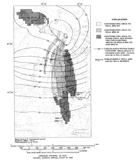
FIGURE 5.1 Contributing areas of wells and ponds in the complex flow system determined by using the three-dimensional model with 1987 average daily pumping rates. (Barlow 1993)
such as maximum prolonged pumping, prevail, and, therefore, conservatively large zones of contribution continue to be used for wellhead protection.
The ground water management experience of Cape Cod has resulted in a better understanding of the resource and the complexity of the aquifer
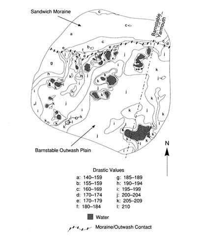
FIGURE 5.2 DRASTIC contours for Zone 1, Barnstable-Yarmouth, Massachusetts.
system, as well as the development of a more ambitious agenda for resource protection. Beginning with goals of protection of existing public water supplies, management interests have grown to include the protection of private wells, potential public supplies, fresh water ponds, and marine embayments. Public concerns over ground water quality have remained high and were a major factor in the creation of the Cape Cod Commission by the Massachusetts legislature. The commission is a land use planning and regulatory agency with broad authority over development projects and the ability to create special resource management areas. The net result of 20 years of effort by many individuals and agencies is the application of
TABLE 5.1 Ranges, Rating, and Weights for DRASTIC Study of Barnstable Outwash Plain Setting (NOTE: gpd/ft 2 = gallons per day per square foot) (Heath 1988)
| Factor | Range | Rating | Weight | Number |
| Depth to Water | 0-50+ feet | 5-10 | 5 | 25-50 |
| Net Recharge Per Year | 10+ inches | 9 | 4 | 36 |
| Aquifer Media | Sand & Gravel | 9 | 3 | 27 |
| Soil Media | Sand | 9 | 2 | 18 |
| Topography | 2-6% | 9 | 1 | 9 |
| Impact of Vadose Zone | Sand & Gravel | 8 | 5 | 40 |
| Hydraulic Conductivity | 2000+ gpd/ft | 10 | 3 | 30 |
|
|
|
|
| Total = 185-210 |
TABLE 5.2 Ranges, Rating, and Weights for DRASTIC Study of Sandwich Moraine Setting (NOTE: gpd/ft 2 = gallons per day per square foot) (Heath 1988)
| Factor | Range | Rating | Weight | Number |
| Depth to Water | 0-100+ feet | 1-10 | 5 | 5-50 |
| Net Recharge Per Year | 10+ inches | 9 | 4 | 36 |
| Aquifer Media | Sand & Gravel | 8 | 3 | 24 |
| Soil Media | Sandy Loam | 6 | 2 | 12 |
| Topography | 6-12% | 5 | 1 | 5 |
| Impact of Vadose Zone | Sand & Gravel | 8 | 5 | 40 |
| Hydraulic Conductivity | 700-1000 gpd/ft | 6 | 3 | 18 |
|
|
|
|
| Total = 140-185 |
higher protection standards to broader areas of the Cape Cod aquifer. With some exceptions for already impaired areas, a differentiated resource protection approach in the vulnerable aquifer setting of Cape Cod has resulted in a program that approaches universal ground water protection.
Florida has 13 million residents and is the fourth most populous state (U.S. Bureau of the Census 1991). Like several other sunbelt states, Florida's population is growing steadily, at about 1,000 persons per day, and is estimated to reach 17 million by the year 2000. Tourism is the biggest industry in Florida, attracting nearly 40 million visitors each year. Ground water is the source of drinking water for about 95 percent of Florida's population; total withdrawals amount to about 1.5 billion gallons per day. An additional 3 billion gallons of ground water per day are pumped to meet the needs of agriculture—a $5 billion per year industry, second only to tourism in the state. Of the 50 states, Florida ranks eighth in withdrawal of fresh ground water for all purposes, second for public supply, first for rural domestic and livestock use, third for industrial/commercial use, and ninth for irrigation withdrawals.
Most areas in Florida have abundant ground water of good quality, but the major aquifers are vulnerable to contamination from a variety of land use activities. Overpumping of ground water to meet the growing demands of the urban centers, which accounts for about 80 percent of the state's population, contributes to salt water intrusion in coastal areas. This overpumping is considered the most significant problem for degradation of ground water quality in the state. Other major sources of ground water contaminants include: (1) pesticides and fertilizers (about 2 million tons/year) used in agriculture, (2) about 2 million on-site septic tanks, (3) more than 20,000 recharge wells used for disposing of stormwater, treated domestic wastewater, and cooling water, (4) nearly 6,000 surface impoundments, averaging one per 30 square kilometers, and (5) phosphate mining activities that are estimated to disturb about 3,000 hectares each year.
The Hydrogeologic Setting
The entire state is in the Coastal Plain physiographic province, which has generally low relief. Much of the state is underlain by the Floridan aquifer system, largely a limestone and dolomite aquifer that is found in both confined and unconfined conditions. The Floridan is overlain through most of the state by an intermediate aquifer system, consisting of predominantly clays and sands, and a surficial aquifer system, consisting of predominantly sands, limestone, and dolomite. The Floridan is one of the most productive aquifers in the world and is the most important source of drinking water for Florida residents. The Biscayne, an unconfined, shallow, limestone aquifer located in southeast Florida, is the most intensively used
aquifer and the sole source of drinking water for nearly 3 million residents in the Miami-Palm Beach coastal area. Other surficial aquifers in southern Florida and in the western panhandle region also serve as sources of ground water.
Aquifers in Florida are overlain by layers of sand, clay, marl, and limestone whose thickness may vary considerably. For example, the thickness of layers above the Floridan aquifer range from a few meters in parts of west-central and northern Florida to several hundred meters in south-central Florida and in the extreme western panhandle of the state. Four major groups of soils (designated as soil orders under the U.S. Soil Taxonomy) occur extensively in Florida. Soils in the western highlands are dominated by well-drained sandy and loamy soils and by sandy soils with loamy subsoils; these are classified as Ultisols and Entisols. In the central ridge of the Florida peninsula, are found deep, well-drained, sandy soils (Entisols) as well as sandy soils underlain by loamy subsoils or phosphatic limestone (Alfisols and Ultisols). Poorly drained sandy soils with organic-rich and clay-rich subsoils, classified as Spodosols, occur in the Florida flatwoods. Organic-rich muck soils (Histosols) underlain by muck or limestone are found primarily in an area extending south of Lake Okeechobee.
Rainfall is the primary source of ground water in Florida. Annual rainfall in the state ranges from 100 to 160 cm/year, averaging 125 cm/year, with considerable spatial (both local and regional) and seasonal variations in rainfall amounts and patterns. Evapotranspiration (ET) represents the largest loss of water; ET ranges from about 70 to 130 cm/year, accounting for between 50 and 100 percent of the average annual rainfall. Surface runoff and ground water discharge to streams averages about 30 cm/year. Annual recharge to surficial aquifers ranges from near zero in perennially wet, lowland areas to as much as 50 cm/year in well-drained areas; however, only a fraction of this water recharges the underlying Floridan aquifer. Estimates of recharge to the Floridan aquifer vary from less than 3 cm/year to more than 25 cm/year, depending on such factors as weather patterns (e.g., rainfall-ET balance), depth to water table, soil permeability, land use, and local hydrogeology.
Permeable soils, high net recharge rates, intensively managed irrigated agriculture, and growing demands from urban population centers all pose considerable threat of ground water contamination. Thus, protection of this valuable natural resource while not placing unreasonable constraints on agricultural production and urban development is the central focus of environmental regulation and growth management in Florida.
Along with California, Florida has played a leading role in the United
States in development and enforcement of state regulations for environmental protection. Detection in 1983 of aldicarb and ethylene dibromide, two nematocides used widely in Florida's citrus groves, crystallized the growing concerns over ground water contamination and the need to protect this vital natural resource. In 1983, the Florida legislature passed the Water Quality Assurance Act, and in 1984 adopted the State and Regional Planning Act. These and subsequent legislative actions provide the legal basis and guidance for the Ground Water Strategy developed by the Florida Department of Environmental Regulation (DER).
Ground water protection programs in Florida are implemented at federal, state, regional, and local levels and involve both regulatory and nonregulatory approaches. The most significant nonregulatory effort involves more than 30 ground water studies being conducted in collaboration with the Water Resources Division of the U.S. Geological Survey. At the state level, Florida statutes and administrative codes form the basis for regulatory actions. Although DER is the primary agency responsible for rules and statutes designed to protect ground water, the following state agencies participate to varying degrees in their implementation: five water management districts, the Florida Geological Survey, the Department of Health and Rehabilitative Services (HRS), the Department of Natural Resources, and the Florida Department of Agriculture and Consumer Services (DACS). In addition, certain interagency committees help coordinate the development and implementation of environmental codes in the state. A prominent example is the Pesticide Review Council which offers guidance to the DACS in developing pesticide use regulation. A method for screening pesticides in terms of their chronic toxicity and environmental behavior has been developed through collaborative efforts of the DACS, the DER, and the HRS (Britt et al. 1992). This method will be used to grant registration for pesticide use in Florida or to seek additional site-specific field data.
Selecting an Approach
The emphasis of the DER ground water program has shifted in recent years from primarily enforcement activity to a technically based, quantifiable, planned approach for resource protection.
The administrative philosophy for ground water protection programs in Florida is guided by the following principles:
Ground water is a renewable resource, necessitating a balance between withdrawals and natural or artificial recharge.
Ground water contamination should be prevented to the maximum degree possible because cleanup of contaminated aquifers is technically or economically infeasible.
It is impractical, perhaps unnecessary, to require nondegradation standards for all ground water in all locations and at all times.
The principle of ''most beneficial use" is to be used in classifying ground water into four classes on the basis of present quality, with the goal of attaining the highest level protection of potable water supplies (Class I aquifers).
Part of the 1983 Water Quality Assurance Act requires Florida DER to "establish a ground water quality monitoring network designed to detect and predict contamination of the State's ground water resources" via collaborative efforts with other state and federal agencies. The three basic goals of the ground water quality monitoring program are to:
Establish the baseline water quality of major aquifer systems in the state,
Detect and predict changes in ground water quality resulting from the effects of various land use activities and potential sources of contamination, and
Disseminate to local governments and the public, water quality data generated by the network.
The ground water monitoring network established by DER to meet the goals stated above consists of two major subnetworks and one survey (Maddox and Spicola 1991). Approximately 1,700 wells that tap all major potable aquifers in the state form the Background Network, which was designed to help define the background water quality. The Very Intensively Studied Area (VISA) network was established to monitor specific areas of the state considered highly vulnerable to contamination; predominant land use and hydrogeology were the primary attributes used to evaluate vulnerability. The DRASTIC index, developed by EPA, served as the basis for statewide maps depicting ground water vulnerability. Data from the VISA wells will be compared to like parameters sampled from Background Network wells in the same aquifer segment. The final element of the monitoring network is the Private Well Survey, in which up to 70 private wells per county will be sampled. The sampling frequency and chemical parameters to be monitored at each site are based on several factors, including network well classification, land use activities, hydrogeologic sensitivity, and funding. In Figure 5.3 , the principal aquifers in Florida are shown along with the distribution of the locations of the monitoring wells in the Florida DER network.
The Preservation 2000 Act, enacted in 1990, mandated that the Land Acquisition Advisory Council (LAAC) "provide for assessing the importance
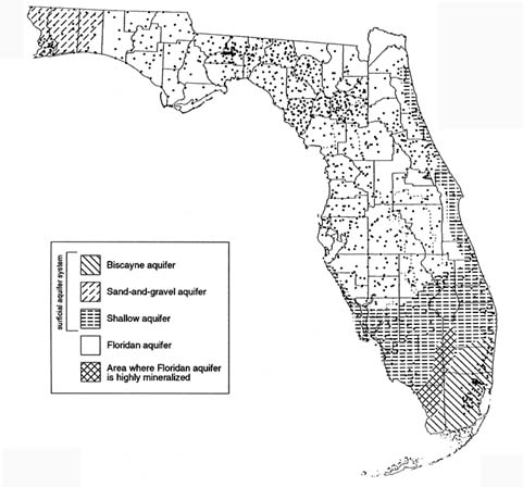
FIGURE 5.3 Principal aquifers in Florida and the network of sample wells as of March 1990 (1642 wells sampled). (Adapted from Maddox and Spicola 1991, and Maddox et al. 1993.)
of acquiring lands which can serve to protect or recharge ground water, and the degree to which state land acquisition programs should focus on purchasing such land." The Ground Water Resources Committee, a subcommittee of the LAAC, produced a map depicting areas of ground water significance at regional scale (1:500,000) (see Figure 5.4 ) to give decision makers the basis for considering ground water as a factor in land acquisition under the Preservation 2000 Act (LAAC 1991). In developing maps for their districts, each of the five water management districts (WMDs) used the following criteria: ground water recharge, ground water quality, aquifer vulnerability, ground water availability, influence of existing uses on the resource, and ground water supply. The specific approaches used by
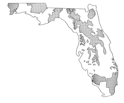
FIGURE 5.4 General areas of ground water significance in Florida. (Map provided by Florida Department of Environmental Regulation, Bureau of Drinking Water and Ground Water Resources.)
the WMDs varied, however. For example, the St. Johns River WMD used a GIS-based map overlay and DRASTIC-like numerical index approach that rated the following attributes: recharge, transmissivity, water quality, thickness of potable water, potential water expansion areas, and spring flow capture zones. The Southwest Florida WMD also used a map overlay and index approach which considered four criteria, and GIS tools for mapping. Existing databases were considered inadequate to generate a DRASTIC map for the Suwannee River WMD, but the map produced using an overlay approach was considered to be similar to DRASTIC maps in providing a general depiction of aquifer vulnerability.
In the November 1988, Florida voters approved an amendment to the Florida Constitution allowing land producing high recharge to Florida's aquifers to be classified and assessed for ad valorem tax purposes based on character or use. Such recharge areas are expected to be located primarily in the upland, sandy ridge areas. The Bluebelt Commission appointed by the 1989 Florida Legislature, studied the complex issues involved and recommended that the tax incentive be offered to owners of such high recharge areas if their land is left undeveloped (SFWMD 1991). The land eligible
for classification as "high water recharge land" must meet the following criteria established by the commission:
The parcel must be located in the high recharge areas designated on maps supplied by each of the five WMDs.
The high recharge area of the parcel must be at least 10 acres.
The land use must be vacant or single-family residential.
The parcel must not be receiving any other special assessment, such as Greenbelt classification for agricultural lands.
Two bills related to the implementation of the Bluebelt program are being considered by the 1993 Florida legislation.
THE SAN JOAQUIN VALLEY
Pesticide contamination of ground water resources is a serious concern in California's San Joaquin Valley (SJV). Contamination of the area's aquifer system has resulted from a combination of natural geologic conditions and human intervention in exploiting the SJV's natural resources. The SJV is now the principal target of extensive ground water monitoring activities in the state.
Agriculture has imposed major environmental stresses on the SJV. Natural wetlands have been drained and the land reclaimed for agricultural purposes. Canal systems convey water from the northern, wetter parts of the state to the south, where it is used for irrigation and reclamation projects. Tens of thousands of wells tap the sole source aquifer system to supply water for domestic consumption and crop irrigation. Cities and towns have sprouted throughout the region and supply the human resources necessary to support the agriculture and petroleum industries.
Agriculture is the principal industry in California. With 1989 cash receipts of more than $17.6 billion, the state's agricultural industry produced more than 50 percent of the nation's fruits, nuts, and vegetables on 3 percent of the nation's farmland. California agriculture is a diversified industry that produces more than 250 crop and livestock commodities, most of which can be found in the SJV.
Fresno County, the largest agricultural county in the state, is situated in the heart of the SJV, between the San Joaquin River to the north and the Kings River on the south. Grapes, stone fruits, and citrus are important commodities in the region. These and many other commodities important to the region are susceptible to nematodes which thrive in the county's coarse-textured soils.
While agricultural diversity is a sound economic practice, it stimulates the growth of a broad range of pest complexes, which in turn dictates greater reliance on agricultural chemicals to minimize crop losses to pests, and maintain productivity and profit. Domestic and foreign markets demand high-quality and cosmetically appealing produce, which require pesticide use strategies that rely on pest exclusion and eradication rather than pest management.
Hydrogeologic Setting
The San Joaquin Valley (SJV) is at the southern end of California's Central Valley. With its northern boundary just south of Sacramento, the Valley extends in a southeasterly direction about 400 kilometers (250 miles) into Kern County. The SJV averages 100 kilometers (60 miles) in width and drains the area between the Sierra Nevada on the east and the California Coastal Range on the west. The rain shadow caused by the Coastal Range results in the predominantly xeric habitat covering the greater part of the valley floor where the annual rainfall is about 25 centimeters (10 inches). The San Joaquin River is the principal waterway that drains the SJV northward into the Sacramento Delta region.
The soils of the SJV vary significantly. On the west side of the valley, soils are composed largely of sedimentary materials derived from the Coastal Range; they are generally fine-textured and slow to drain. The arable soils of the east side developed on relatively unweathered, granitic sediments. Many of these soils are wind-deposited sands underlain by deep coarse-textured alluvial materials.
From the mid-1950s until 1977, dibromochloropropane (DBCP) was the primary chemical used to control nematodes. DBCP has desirable characteristics for a nematocide. It is less volatile than many other soil fumigants, such as methylbromide; remains active in the soil for a long time, and is effective in killing nematodes. However, it also causes sterility in human males, is relatively mobile in soil, and is persistent. Because of the health risks associated with consumption of DBCP treated foods, the nematocide was banned from use in the United States in 1979. After the ban, several well water studies were conducted in the SJV by state, county and local authorities. Thirteen years after DBCP was banned, contamination of well waters by the chemical persists as a problem in Fresno County.
Public concern over pesticides in ground water resulted in passage of the California Pesticide Contamination Prevention Act (PCPA) of 1985. It is a broad law that establishes the California Department of Pesticide Regulation
as the lead agency in dealing with issues of ground water contamination by pesticides. The PCPA specifically requires:
pesticide registrants to collect and submit specific chemical and environmental fate data (e.g., water solubility, vapor pressure, octanol-water partition coefficient, soil sorption coefficient, degradation half-lives for aerobic and anaerobic metabolism, Henry's Law constant, hydrolysis rate constant) as part of the terms for registration and continued use of their products in California.
establishment of numerical criteria or standards for physical-chemical characteristics and environmental fate data to determine whether a pesticide can be registered in the state that are at least as stringent as those standards set by the EPA,
soil and water monitoring investigations be conducted on:
pesticides with properties that are in violation of the physical-chemical standards set in 2 above, and
pesticides, toxic degradation products or other ingredients that are:
contaminants of the state's ground waters, or
found at the deepest of the following soil depths:
2.7 meters (8 feet) below the soil surface,
below the crop root zone, or
below the microbial zone, and
creation of a database of wells sampled for pesticides with a provision requiring all agencies to submit data to the California Department of Pesticide Regulation (CDPR).
Difficulties associated with identifying the maximum depths of root zone and microbial zone have led to the establishment of 8 feet as a somewhat arbitrary but enforceable criterion for pesticide leaching in soils.
Selection and Implementation of an Approach
Assessment of ground water vulnerability to pesticides in California is a mechanical rather than a scientific process. Its primary goal is compliance with the mandates established in the PCPA. One of these mandates requires that monitoring studies be conducted in areas of the state where the contaminant pesticide is used, in other areas exhibiting high risk portraits (e.g., low organic carbon, slow soil hydrolysis, metabolism, or dissipation), and in areas where pesticide use practices present a risk to the state's ground water resources.
The numerical value for assessments was predetermined by the Pesticide Use Report (PUR) system employed in the state. Since the early
1970s, California has required pesticide applicators to give local authorities information on the use of restricted pesticides. This requirement was extended to all pesticides beginning in 1990. Application information reported includes names of the pesticide(s) and commodities, the amount applied, the formulation used, and the location of the commodity to the nearest section (approximately 1 square mile) as defined by the U.S. Rectangular Coordinate System. In contrast to most other states that rely on county pesticide sales in estimating pesticide use, California can track pesticide use based on quantities applied to each section. Thus, the section, already established as a political management unit, became the basic assessment unit.
The primary criteria that subject a pesticide to investigation as a ground water pollutant are:
detection of the pesticide or its metabolites in well samples, or
its failure to conform to the physical-chemical standards set in accordance with the PCPA, hence securing its position on the PCPA's Ground Water Protection List of pesticides having a potential to pollute ground water.
In either case, relatively large areas surrounding the original detection site or, in the latter case, high use regions are monitored via well surveys. Positive findings automatically increase the scope of the surveys, and since no tolerance levels are specified in the PCPA, any detectable and confirmed result establishes a pesticide as a contaminant.
When a pesticide or its degradation products is detected in a well water sample and the pesticide is judged to have contaminated the water source as a result of a legal agricultural use, the section the well is in is declared a Pesticide Management Zone (PMZ). Further application of the detected pesticide within PMZ boundaries may be prohibited or restricted, depending on the degree of contamination and subject to the availability of tried and tested modifications in management practices addressing environmental safety in use of the pesticide. PMZs are pesticide-specific—each contaminant pesticide has its own set of PMZs which may or may not overlap PMZs assigned another pesticide. Currently, consideration is being given to the extension of PMZs established for one chemical to other potential pesticide pollutants. In addition to monitoring activities in PMZs, protocols have been written to monitor ground water in sections adjacent to a PMZ. Monitoring of adjacent sections has resulted in many new PMZs. Currently, California has 182 PMZs involving five registered pesticides.
California has pursued this mechanical approach to assessing ground water vulnerability to pesticides for reasons that cover a spectrum of political, economic, and practical concerns. As noted earlier, the scale of the assessment unit was set at the section level because it is a well-defined
geopolitical unit used in the PUR system. Section boundaries frequently are marked by roads and highways, which allows the section to be located readily and makes enforcement of laws and regulations more practical. California law also requires that well logs be recorded by drillers for all wells in the state. Well-site information conforms to the U.S. Rectangular Coordinate System's township, range, and section system.
The suitability and reliability of databases available for producing vulnerability assessments was a great concern before passage of the PCPA in 1985. Soil survey information holds distinct advantages for producing assessments and developing best management practices strategies, but it was not available in a format that could work in harmony with PUR sections. To date, several areas of the SJV are not covered by a modern soil survey; they include the western part of Tulare County, which contains 34 PMZs. Other vadose zone data were sparse, it available at all.
The use of models was not considered appropriate, given the available data and because no single model could cope with the circumstances in which contaminated ground water sources were being discovered in the state. While most cases of well contamination were associated with the coarse-textured soils of the SJV and the Los Angeles Basin, several cases were noted in areas of the Central Valley north of the SJV, where very dense fine-textured soils (vertisols and other cracking clays) were dominant.
The potential vagaries and uncertainties associated with more scientific approaches to vulnerability assessment, given the tools available when the PCPA was enacted, presented too large a risk for managers to consider endorsing their use. In contrast, the basic definition of the PMZ is difficult to challenge (pesticide contamination has been detected or not detected) in the legal sense. And the logic of investing economic resources in areas immediately surrounding areas of acknowledged contamination are relatively undisputable. The eastern part of the SJV contains more than 50 percent of the PMZs in the state. Coarse-textured soils of low carbon content are ubiquitous in this area and are represented in more than 3,000 sections. The obvious contamination scenario is the normal scenario in the eastern SJV, and because of its size it creates a huge management problem. While more sophisticated methods for assessing ground water vulnerability have been developed, a question that begs to be asked is "How would conversion to the use of enhanced techniques for evaluating ground water vulnerability improve ground water protection policy and management in the SJV?"
More than 90 percent of the population of Hawaii depends on ground water (nearly 200 billion gallons per day) for their domestic supply (Au 1991). Ground water contamination is of special concern in Hawaii, as in other insular systems, where alternative fresh water resources are not readily available or economically practical. Salt water encroachment, caused by pumping, is by far the biggest source of ground water contamination in Hawaii; however, nonpoint source contamination from agricultural chemicals is increasingly a major concern. On Oahu, where approximately 80 percent of Hawaii's million-plus population resides, renewable ground water resources are almost totally exploited; therefore, management action to prevent contamination is essential.
Each of the major islands in the Hawaiian chain is formed from one or more shield volcanoes composed primarily of extremely permeable thin basaltic lava flows. On most of the Hawaiian islands the margins of the volcanic mountains are overlapped by coastal plain sediments of alluvial and marine origin that were deposited during periods of volcanic quiescence. In general, the occurrence of ground water in Hawaii, shown in Figure 5.5 , falls into three categories: (1) basal water bodies floating on and displacing salt water, (2) high-level water bodies impounded within compartments formed by impermeable dikes that intrude the lava flows, and (3) high-level water bodies perched on ash beds or soils interbedded with
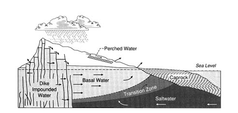
FIGURE 5.5 Cross section of a typical volcanic dome showing the occurrence of ground water in Hawaii (After Peterson 1972. Reprinted, by permission, from Water Well Journal Publishing Company, 1972.)
thin lava flows on unconformities or on other relatively impervious lava flows (Peterson 1972).
A foundation of the tourist industry in Hawaii is the pristine environment. The excellent quality of Hawaii's water is well known. The public has demanded, and regulatory agencies have adopted, a very conservative, zero-tolerance policy on ground water contamination. The reality, however, is that past, present, and future agricultural, industrial, and military activities present potentially significant ground water contamination problems in Hawaii.
Since 1977 when 1,874 liters of ethylene dibromide (EDB) where spilled within 18 meters of a well near Kunia on the island of Oahu, the occurrence and distribution of contaminants in Hawaii's ground water has been carefully documented by Oki and Giambelluca (1985, 1987) and Lau and Mink (1987). Before 1981, when the nematocide dibromochloropropane (DBCP) was found in wells in central Oahu, the detection limit for most chemicals was too high to reveal the low level of contamination that probably had existed for many years.
Concern about the fate of agriculture chemicals led the Hawaii State Department of Agriculture to initiate a large sampling program to characterize the sources of nonpoint ground water contamination. In July 1983, 10 wells in central Oahu were closed because of DBCP and EDB contamination. The public has been kept well informed of possible problems through the publication of maps of chemicals detected in ground water in the local newspaper. Updated versions of these maps are shown in Figures 5.6a , b , c , and d .
In Hawaii, interagency committees, with representation from the Departments of Health and Agriculture, have been formed to address the complex technical and social questions associated with ground water contamination from agricultural chemicals. The Hawaii legislature has provided substantial funding to groups at the University of Hawaii to develop the first GIS-based regional scale chemical leaching assessment approach to aid in pesticide regulation. This effort, described below, has worked to identify geographic areas of concern, but the role the vulnerability maps generated by this system will play in the overall regulatory process is still unclear.
Agrichemicals are essential to agriculture in Hawaii. It is not possible to maintain a large pineapple monoculture in Hawaii without nematode control using pesticides. Pineapple and sugar growers in Hawaii have generally employed well controlled management practices in their use of fertilizers, herbicides, and insecticides. In the early 1950s, it was thought that organic chemicals such as DBCP and EDB would not leach to ground water
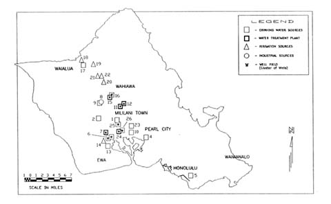
FIGURE 5.6a The occurrence and distribution of ground water contamination on the Island of Oahu. (Map provided by Hawaii State Department of Health.)
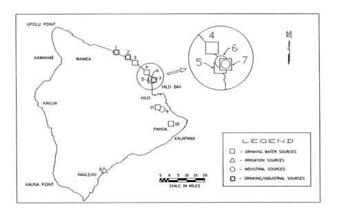
FIGURE 5.6b The occurrence and distribution of ground water contamination on the Island of Hawaii. (Map provided by Hawaii State Department of Health.)
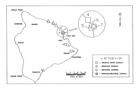
FIGURE 5.6c The occurrence and distribution of ground water contamination on the Island of Maui. (Map provided by Hawaii State Department of Health.)
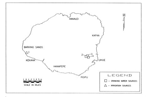
FIGURE 5.6d The occurrence and distribution of ground water contamination on the Island of Kauai. (Map provided by Hawaii State Department of Health.)
because (1) the chemicals are highly sorbed in soils with high organic carbon contents, (2) the chemicals are highly volatile, and (3) the water table is several hundred meters below the surface. Measured concentrations of DBCP and EDB down to 30 meters at several locations have shown the original assessment to be wrong. They have resulted in an urgent need to understand processes such as preferential flow better and to predict if the replacement chemicals used today, such as Telon II, will also leach to significant depths.
Leaching of pesticides to ground water in Hawaii could take decades. This time lag could lead to a temporary false sense of security, as happened in the past and potentially result in staggering costs for remedial action. For this reason, mathematical models that permit the user to ask ''what if" questions have been developed to help understand what the future may hold under certain management options. One needs to know what the fate of chemicals applied in the past will be and how to regulate the chemicals considered for use in the future; models are now being developed and used to help make these vulnerability assessments.
Researchers have embarked on several parallel approaches to quantitatively assess the vulnerability of Hawaii's ground water resources, including: (1) sampling, (2) physically-based numerical modeling, and (3) vulnerability mapping based on a simple chemical leaching index. Taken together these approaches have provided insight and guidance for work on a complex, spatially and temporally variable problem.
The sampling programs (Wong 1983 and 1987, Peterson et al. 1985) have shown that the chemicals applied in the past do, in fact, leach below the root zone, contrary to the original predictions, and can eventually reach the ground water. Experiments designed to characterize the nuances of various processes, such as volatilization, sorption, and degradation, have been conducted recently and will improve the conceptualization of mathematical models in the future.
The EPA's Pesticide Root Zone Model (PRZM), a deterministic-empirical/conceptual fluid flow/solute transport model, has been tested by Loague and co-workers (Loague et al. 1989a, b; Loague 1992) against measured concentration profiles for DBCP and EDB in central Oahu. These simulations illustrate that the chemicals used in the past can indeed move to considerable depths. Models of this kind, once properly validated, can be used to simulate the predicted fate of future pesticide applications. One must always remember, however, that numerical simulations must be interpreted in terms of the limiting assumptions associated with model and data errors.
Ground water vulnerability maps and assessments of their uncertainty were pioneered at the University of Hawaii in the Department of Agriculture Engineering (Khan and Liang 1989, Loague and Green 1990a). These pesticide leaching assessments were made by coupling a simple mobility index to a geographic information system. Loague and coworkers have investigated the uncertainty in these maps owing to data and model errors (Loague and Green 1988; Loague et al. 1989c, 1990; Loague and Green 1990b, 1990c; Loague 1991; Kleveno et al. 1992; Yost et al. 1993). The Hawaiian database on soils, climate, and chemicals is neither perfect nor poor for modeling applications; it is typical of what exists in most states—major extrapolations are required to estimate the input parameters required for almost any chemical fate model.
Sampling from wells in Hawaii has shown the concentrations of various chemicals, both from agriculture and industrial sources, which have leached to ground water in Hawaii. These concentrations, in general, are low compared to the levels detected in other states and for the most part are below health advisory levels established by EPA. In some instances contamination has not resulted from agriculture, but rather from point sources such as chemical loading and mixing areas and possibly from ruptured fuel lines. The widespread presence of trichloropropane (TCP) in Hawaii's ground water and deep soil cores at concentrations higher than DBCP was totally unexpected. TCP was never applied as a pesticide, but results from the manufacture of the fumigant DD, which was used until 1977 in pineapple culture. The occurrence of TCP illustrates that one must be aware of the chemicals applied as well as their components and transformation products.
Wells have been closed in Hawaii even though the measured contaminant concentrations have been below those considered to pose a significant health risk. At municipal well locations in central Oahu, where DBCP, EDB, and/or TCP have been detected, the water is now passed through carbon filters before it is put into the distribution system. The cost of this treatment is passed on to the water users, rather than to those who applied the chemicals.
The pesticide leaching assessment maps developed by Khan and Liang (1989) are intended for incorporation into the regulatory process. Decisions are not made on the basis of the red and green shaded areas for different chemicals (see Plate 3 ), but this information is considered. The uncertainty analysis by Loague and coworkers has shown some of the limitations of deterministic assessments in the form of vulnerability maps and provided initial guidance on data shortfalls.
APPLICATION OF A VULNERABILITY INDEX FOR DECISION-MAKING AT THE NATIONAL LEVEL
Need for a vulnerability index.
A vulnerability index for ground water contamination by pesticides has been developed and used by USDA as a decision aid to help attain the objectives of the President's Water Quality Initiative (see Box 1.1 ). A vulnerability index was needed for use in program management and to provide insight for policy development. Motivation for the development of the vulnerability index was provided by two specific questions:
Given limited resources and the geographic diversity of the water quality problems associated with agricultural production, what areas of the country have the highest priority for study and program implementation?
What policy implications emerge from the spatial patterns of the potential for conamination from a national perspective, given information currently available about farming practices and chemical use in agriculture?
Description of the Vulnerability Index
A vulnerability index was derived to evaluate the likelihood of shallow ground water contamination by pesticides used in agriculture in one area compared to another area. Because of the orientation of Initiative policies to farm management practices, it was necessary that the vulnerability measure incorporate field level information on climate, soils, and chemical use. It also needed to be general enough to include all areas of the country and all types of crops grown.
A Ground Water Vulnerability Index for Pesticides (GWVIP) was developed by applying the Soil-Pesticide Interaction Screening Procedure (SPISP) developed by the Soil Conservation Service to the National Resource Inventory (NRI) land use database for 1982 and the state level pesticide use database created by Resources for the Future (Gianessi and Puffer 1991). Details of the computational scheme and databases used are described by Kellogg et al. (1992). The 1982 NRI and the associated SOIL-5 database provide information on soil properties and land use at about 800,000 sample points throughout the continental United States. This information is sufficient to apply the SPISP to each point and thus obtain a relative measure of the soil leaching potential throughout the country. The RFF pesticide use database was used to infer chemical use at each point on the basis of the crop type recorded in the NRI database. By taking advantage of the statistical properties of the NRI database, which is based on a statistical survey
sampling design, the GWVIP score at each of the sample points can be statistically aggregated for making comparisons among regions.
Since the GWVIP is an extension of a screening procedure, it is designed to minimize the likelihood of incorrectly identifying an area as having a low potential for contamination—that is, false negatives are minimized and false positives are tolerated. The GWVIP is designed to classify an area as having a potential problem even if the likelihood is small.
GWVIP scores were graphically displayed after embedding them in a national cartographic database consisting of 13,172 polygons created by overlaying the boundaries of 3,041 counties, 189 Major Land Resource Areas (MLRAs), 2,111 hydrologic units, and federal lands.
Three caveats are especially important in using the GWVIP and its aggregates as a decision aid:
Land use data are for 1982 and do not represent current cropping patterns in some parts of the country. Although total cropland acreage has remained fairly stable over the past 10 years, there has been a pronounced shift from harvested cropland to cropland idled in government programs.
The approach uses a simulation model that predicts the amount of chemical that leaches past the root zone. In areas where the water table is near the surface, these predictions relate directly to shallow ground water contamination. In other areas a time lag is involved. No adjustment was made for areas with deep water tables.
No adjustment in chemical use is made to account for farm management factors, such as chemical application rates and crop rotations. The approach assumes that chemical use is the same for a crop grown as part of a rotation cropping system as for continuous cropping. Since the chemical use variable in the GWVIP calculation is based on acres of land treated with pesticides, application rates are also not factored into the analysis.
Application to Program Management
By identifying areas of the country that have the highest potential for leaching of agrichemicals, the GWVIP can serve as a basis for selecting sites for implementation of government programs and for more in-depth research on the environmental impact of agrichemical use. These sites cannot be selected exclusively on the basis of the GWVIP score, however, because other factors, such as surface water impacts and economic and demographic factors, are also important.
For example, the GWVIP has been used as a decision aid in selecting sites for USDA's Area Study Program, which is designed to provide chemical use and farming practice information to aid in understanding the relationships among farming activities, soil properties, and ground water quality.
The National Agricultural Statistics Service interviews farm operators in 12 major watersheds where the U.S. Geological Survey is working to measure the quality of surface and ground water resources under its National Water Quality Assessment Program. At the conclusion of the project, survey information will be combined with what is learned in other elements of the President's Water Quality Initiative to assess the magnitude of the agriculture-related water quality problem for the nation as a whole and used to evaluate the potential economic and environmental effects of Initiative policies of education, technical assistance, and financial assistance if implemented nationwide.
To meet these objectives, each Area Study site must have a high potential for ground water contamination relative to other areas of the country. A map showing the average GWVIP for each of the 13,172 polygons comprising the continental United States, shown in Plate 3 , was used to help select the sites. As this map shows, areas more likely to have leaching problems with agrichemicals than other areas of the country occur principally along the coastal plains stretching from Alabama and Georgia north to the Chesapeake Bay area, the corn belt states, the Mississippi River Valley, and the irrigated areas in the West. Sites selected for study in 1991 and 1992 include four from the eastern coastal plain (Delmarva Peninsula, southeastern Pennsylvania, Virginia and North Carolina, and southern Georgia), four from the corn belt states (Nebraska, Iowa, Illinois, and Indiana), and two from the irrigated areas in the West (eastern Washington and southeastern Idaho). Four additional sites will be selected for study in 1993.
Application to Policy Analysis and Development
The GWVIP has also been used by USDA to provide a national perspective on agricultural use of pesticides and the potential for ground water contamination to aid in policy analysis and development.
The geographic distribution of GWVIP scores has shown that the potential for ground water contamination is diverse both nationally and regionally. Factors that determine intrinsic vulnerability differ in virtually every major agricultural region of the country. Whether an impact is realized in these intrinsically vulnerable areas depends on the activities of producers—such as the type of crop planted, chemical use, and irrigation practices—which also vary both nationally and regionally. High vulnerability areas are those where a confluence of these factors is present. But not all cropland is vulnerable to leaching. About one-fourth of all cropland has GWVIP scores that indicate very low potential for ground water contamination from the use of agrichemicals. Nearly all agricultural states have significant acreage that meets this low vulnerability criterion. Areas of the country identified as being in a high vulnerability group relative to potential
for agrichemical leaching also have significant acreages that appear to have low vulnerability.
This mix of relative vulnerabilities both nationally and regionally has important policy implications. With the potential problem so diverse, it is not likely that simple, across-the-board solutions will work. Simple policies—such as selective banning of chemicals—may reduce the potential for ground water contamination in problem areas while imposing unnecessary costs on farming in nonproblem areas. The geographic diversity of the GWVIP suggests that the best solutions will come from involvement of both local governments and scientists with their state and national counter-parts to derive policies that are tailored to the unique features of each problem area.
In the future, USDA plans to use vulnerability indexes, like the GWVIP, in conjunction with economic models to evaluate the potential for solving agriculture-related water quality problems with a nationwide program to provide farmers with the knowledge and technical means to respond voluntarily to water quality concerns.
These six case studies illustrate how different approaches to vulnerability assessment have evolved under diverse sets of management requirements, data constraints, and other technical considerations. In addition, each of these examples shows that vulnerability assessment is an ongoing process through which information about a region's ground water resources and its quality can be organized and examined methodically.
In Iowa, the Iowa DNR staff elected to keep their vulnerability characterization efforts as simple as possible, and to use only properties for which data already existed or could be easily checked. They assumed that surficial features such as the soil are too thin and too disrupted by human activities (e.g., tillage, abandoned wells) to provide effective ground water protection at any particular location and sought to identify a surrogate measure for average travel time from the land surface to the aquifer. Thus, a ground water vulnerability map was produced which represents vulnerability primarily on the basis of depth to ground water and extent of overlying materials. Wells and sinkholes are also shown. The results are to be used for informing resource managers and the public of the vulnerability of the resource and to determine the type of information most needed to develop an even better understanding of the vulnerability of Iowa's ground water.
The Cape Cod approach to ground water vulnerability assessment is perhaps one of the oldest and most sophisticated in the United States. Driven by the need to protect the sole source drinking water aquifer underlying this sandy peninsula, the vulnerability assessment effort has focused on the identification
and delineation of the primary recharge areas for the major aquifers. This effort began with a simple mass balance approach which assumed even recharge within a circular area around each drinking water well. It has since evolved to the development of a complex, particle-tracking three-dimensional model that uses site-specific data to delineate zones of contribution. Bolstered by strong public concern, Cape Cod has been able to pursue an ambitious and sophisticated agenda for resource protection, and now boasts a sophisticated differential management ground water protection program.
In Florida, ground water resource managers rely on a combination of monitoring and vulnerability assessment techniques to identify high recharge areas the develop the state ground water protection program. Overlay and index methods, including several modified DRASTIC maps were produced to identify areas of ground water significance in support of decision making in state land acquisition programs aimed at ground water protection. In addition, several monitoring networks have been established to assess background water quality and monitor actual effects in areas identified as highly vulnerable. The coupling of ground water vulnerability assessments with monitoring and research efforts, provides the basis of an incremental and evolving ground water protection program in Florida.
The programs to protect ground water in California's intensely agricultural San Joaquin Valley are driven largely by compliance with the state Pesticide Contamination Prevention Act. The California Department of Pesticide Regulation determined that no model would be sufficient to cover their specific regulatory needs and that the available data bases were neither suitable nor reliable for regulatory purposes. Thus, a ground water protection program was built on the extensive existing pesticide use reporting system and the significant ground water monitoring requirements of the act. Using farm sections as management units, the state declares any section in which a pesticide or its degradation product is detected as a pesticide management zone and establishes further restrictions and monitoring requirements. Thus, the need to devise a defensible regulatory approach led California to pursue a mechanistic monitoring based approach rather than a modeling approach that would have inherent and difficult to quantify uncertainties.
In contrast, the approach taken in Hawaii involves an extensive effort to understand the uncertainty associated with the assessment models used. The purpose of this is to provide guidance to, but not the sole basis for, the pesticide regulation program. The combined use of sampling, physically-based numerical modeling, and a chemical leaching index has led to extensive improvements in the understanding of the fate of pesticides in the subsurface environment. Uncertainty analyses are used to determine where additional information would be most useful.
Finally, USDA's Ground Water Vulnerability Index for Pesticides illustrates a national scale vulnerability assessment developed for use as a decision aid and analytical tool for national policies regarding farm management and water quality. This approach combines nationally available statistical information on pesticide usage and soil properties with a simulation model to predict the relative likelihood of contamination in cropland areas. USDA has used this approach to target sites for its Area Study Program which is designed to provide information to farmers about the relationships between farm management practices and water quality. The results of the GWVIP have also indicated that, even at the regional level, there is often an mix of high and low vulnerability areas. This result suggests that effective ground water policies should be tailored to local conditions.
Au, L.K.L. 1991. The Relative Safety of Hawaii's Drinking Water. Hawaii Medical Journal 50(3): 71-80.
Barlow, P.M. 1993. Particle-Tracking Analysis of Contributing Areas of Public-Supply Wells in Simple and Complex Flow Systems, Cape Cod, Massachusetts. USGS Open File Report 93-159. Marlborough, Massachusetts: U.S. Geological Survey.
Britt, J.K., S.E. Dwinell, and T.C. McDowell. 1992. Matrix decision procedure to assess new pesticides based on relative ground water leaching potential and chronic toxicity. Environ. Toxicol. Chem. 11: 721-728.
Cape Cod Commission (CCC). 1991. Regional Policy Plan. Barnstable, Massachusetts: Cape Cod Commission.
Cape Cod Planning and Economic Development Commission (CCPEDC). March 1978a. Draft Area Wide Water Quality Management Plan for Cape Cod. Barnstable, Massachusetts: Cape Cod Commission.
Cape Cod Planning and Economic Development Commission (CCPEDC). September 1978b. Final Area Wide Water Quality Management Plan for Cape Cod. Barnstable, Massachusetts: Cape Cod Commission.
Department of Environmental Protection, Division of Water Supply (DEP-WS). 1991. Guidelines and Policies for Public Water Supply Systems. Massachusetts Department of Environmental Protection.
Gianessi, L.P., and C.A. Puffer. 1991. Herbicide Use in the United States: National Summary Report. Washington, D.C.: Resources for the Future.
Guswa, J.H., and D.R. LeBlanc. 1981. Digital Models of Ground water Flow in the Cape Cod Aquifer System, MA. USGS Water Supply Paper 2209. U.S. Geological Survey.
Heath, D.L. 1988. DRASTIC mapping of aquifer vulnerability in eastern Barnstable and western Yarmouth, Cape Cod, Massachusetts. In Appendix D, Cape Cod Aquifer Management Project, Final Report, G.A. Zoto and T. Gallagher, eds. Boston: Massachusetts Department of Environmental Quality Engineering.
Horsely, S.W. 1983. Delineating zones of contribution of public supply wells to protect ground water . In Proceedings of the National Water Well Association Eastern Regional Conference, Ground-Water Management, Orlando, Florida.
Hoyer, B.E. 1991. Ground water vulnerability map of Iowa. Pp. 13-15 in Iowa Geology, no. 16. Iowa City, Iowa: Iowa Department of Natural Resources.
Hoyer, B.E., J.E. Combs, R.D. Kelley, C. Cousins-Leatherman, and J.H. Seyb. 1987. Iowa Ground water Protection Strategy. Des Moines: Iowa Department of Natural Resources.
Kellogg, R.L., M.S. Maizel, and D.W. Goss. 1992. Agricultural Chemical Use and Ground Water Quality: Where Are the Potential Problems? Washington, D.C.: U.S. Department of Agriculture, Soil Conservation Service.
Khan, M.A., and T. Liang. 1989. Mapping pesticide contamination potential. Environmental Management 13(2):233-242.
Kleveno, J.J., K. Loague, and R.E. Green. 1992. An evaluation of a pesticide mobility index: Impact of recharge variation and soil profile heterogeneity. Journal of Contaminant Hydrology 11(1-2):83-99.
Land Acquisition Advisory Council (LAAC). 1991. Ground Water Resources Committee Final Report: Florida Preservation 2000 Needs Assessment. Tallahassee, Florida: Department of Environmental Regulation. 39 pp.
Lau, L.S., and J.F. Mink. 1987. Organic contamination of ground water: A learning experience. J. American Water Well Association 79(8):37-42.
LeBlanc, D.R., and J.H. Guswa. 1977. Water-Table Map of Cape Cod, MA. May 23-27, 1976, USGS Open File Report 77-419, scale 1:48,000.
Loague, K. 1991. The impact of land use on estimates of pesticide leaching potential: Assessments and uncertainties. Journal of Contaminant Hydrology 8: 157-175.
Loague, K. 1992. Simulation of organic chemical movement in Hawaii soils with PRZM: 3. Calibration. Pacific Science 46(3):353-373.
Loague, K.M., and R.E. Green. 1988. Impact of data-related uncertainties in a pesticide leaching assessment. Pp. 98-119 in Methods for Ground Water Quality Studies, D.W. Nelson and R.H. Dowdy, eds. Lincoln, Nebraska: Agricultural Research Division, University of Nebraska.
Loague, K., and R.E. Green. 1990a. Comments on "Mapping pesticide contamination potential," by M.A. Khan and T. Liang. Environmental Management 4:149-150.
Loague, K., and R.E. Green. 1990b. Uncertainty in Areal Estimates of Pesticide Leaching Potential. Pp. 62-67 in Transactions of 14th International Congress of Soil Science. Kyoto, Japan: International Soil Science Society.
Loague, K., and R.E. Green. 1990c. Criteria for evaluating pesticide leaching models. Pp. 175-207 in Field-Scale Water and Solute Flux in Soils, K. Roth, H. Flühler, W.A. Jury, and J.C. Parker, eds. Basel, Switzerland: Birkhauser Verlag.
Loague, K.M., R.E. Green, C.C.K. Liu, and T.C. Liang. 1989a. Simulation of organic chemical movement in Hawaii soils with PRZM: 1. Preliminary results for ethylene dibromide. Pacific Science 43(1):67-95.
Loague, K., T.W. Giambelluca, R.E. Green, C.C.K. Liu, T.C. Liang, and D.S. Oki. 1989b. Simulation of organic chemical movement in Hawaii soils with PRZM: 2. Predicting deep penetration of DBCP, EDB, and TCP. Pacific Science 43(4):362-383.
Loague, K.M., R.S. Yost, R.E. Green, and T.C. Liang. 1989c. Uncertainty in a pesticide leaching assessment for Hawaii. Journal of Contaminant Hydrology 4:139-161.
Loague, K., R.E. Green, T.W. Giambelluca, T.C. Liang, and R.S. Yost. 1990. Impact of uncertainty in soil, climatic, and chemical information in a pesticide leaching assessment. Journal of Contaminant Hydrology 5:171-194.
Maddox, G., and J. Spicola. 1991. Ground Water Quality Monitoring Network. Tallahassee, Florida: Florida Department of Environmental Regulation. 20 pp.
Maddox, G., J. Lloyd, T. Scott, S. Upchurch, and R. Copeland, eds. 1993. Florida's Ground Water Quality monitoring Program: Background Hydrogeochemistry. Florida Geological Survey Special Publication #34. Tallahassee, Florida: Florida Department of Environmental Regulation in cooperation with Florida Geological Survey.
National Research Council (NRC). 1986. Ground Water Quality Protection: State and Local Strategies. Washington, D.C.: National Academy Press.
Oki, D.S., and T.W. Giambelluca. 1985. Subsurface Water and Soil Quality Data Base for State of Hawaii: Part 1. Spec. Rept. 7. Manoa, Hawaii: Water Resources Research Center, University of Hawaii at Manoa.
Oki, D.S., and T.W. Giambelluca. 1987. DBCP, EDB, and TCP contamination of ground water in Hawaii. Ground Water 25:693-702.
Olimpio, J.C., E.C. Flynn, S. Tso, and P.A. Steeves. 1991. Use of a Geographic Information System to Assess Risk to Ground-Water Quality at Public-Supply Wells, Cape Cod, Massachusetts. Boston, Massachusetts: U.S. Geological Survey.
Peterson, F.L. 1972. Water development on tropic volcanic islands—Type example: Hawaii. Ground Water 5:18-23.
Peterson, F.L., K.R. Green, R.E. Green, and J.N. Ogata. 1985. Drilling program and pesticide analysis of core samples from pineapple fields in central Oahu. Water Resources Research Center, University of Hawaii at Manoa, Special Report 7.5. Photocopy.
Southwest Florida Water Management Districts (SFWMD). 1991. The Bluebelt Commission. Brooksville, Florida: Southwest Florida Water Management Districts.
U.S. Bureau of the Census. 1991. Statistical Abstracts of the United States: 1991, 111th edition. Washington, D.C.: U.S. Government Printing Office.
Wong, L. 1983. Preliminary report on soil sampling EDB on Oahu. Pesticide Branch, Div. of Plant Industry, Department of Agriculture, State of Hawaii. Photocopy.
Wong, L. 1987. Analysis of ethylene dibromide distribution in the soil profile following shank injection for nematode control in pineapple culture. Pp. 28-40 in Toxic Organic Chemicals in Hawaii's Water Resources, P.S.C. Rao and R.E. Green, eds. Ser. 086. Honolulu: Hawaii Inst. Trop Agric. Hum. Resources Res. Exten. University of Hawaii.
Yost, R.S., K. Loague, and R.E. Green. 1993. Reducing variance in soil organic carbon estimates—soil classification and geostatistical approaches. Geoderma 57(3):247-262
Since the need to protect ground water from pollution was recognized, researchers have made progress in understanding the vulnerability of ground water to contamination. Yet, there are substantial uncertainties in the vulnerability assessment methods now available.
With a wealth of detailed information and practical advice, this volume will help decision-makers derive the most benefit from available assessment techniques. It offers:
- Three laws of ground water vulnerability.
- Six case studies of vulnerability assessment.
- Guidance for selecting vulnerability assessments and using the results.
- Reviews of the strengths and limitations of assessment methods.
- Information on available data bases, primarily at the federal level.
This book will be indispensable to policymakers and resource managers, environmental professionals, researchers, faculty, and students involved in ground water issues, as well as investigators developing new assessment methods.
READ FREE ONLINE
Welcome to OpenBook!
You're looking at OpenBook, NAP.edu's online reading room since 1999. Based on feedback from you, our users, we've made some improvements that make it easier than ever to read thousands of publications on our website.
Do you want to take a quick tour of the OpenBook's features?
Show this book's table of contents , where you can jump to any chapter by name.
...or use these buttons to go back to the previous chapter or skip to the next one.
Jump up to the previous page or down to the next one. Also, you can type in a page number and press Enter to go directly to that page in the book.
Switch between the Original Pages , where you can read the report as it appeared in print, and Text Pages for the web version, where you can highlight and search the text.
To search the entire text of this book, type in your search term here and press Enter .
Share a link to this book page on your preferred social network or via email.
View our suggested citation for this chapter.
Ready to take your reading offline? Click here to buy this book in print or download it as a free PDF, if available.
Get Email Updates
Do you enjoy reading reports from the Academies online for free ? Sign up for email notifications and we'll let you know about new publications in your areas of interest when they're released.
- Agriculture
- Environmental Pollution
- Environmental Science
- Water Pollution
Water Pollution: Sources and Its Impact on Human Health, Control and Managing
- Journal of International Cooperation and Development 5(1):69
- CC BY-NC 4.0

- Jilin University
- This person is not on ResearchGate, or hasn't claimed this research yet.
Discover the world's research
- 25+ million members
- 160+ million publication pages
- 2.3+ billion citations
- Aanchal Eusebius

- Kartikeya Shukla
- Priyanka Singh

- Steven Kenway
- Ilje Pikaar
- Irdayanti Mat Nashir

- Nor Asniza Ishak
- INT J ENVIRON AN CH
- Nnabuk Eddy Okon
- Akhilesh Kumar Yadav

- CHEMOSPHERE

- Amrik Bhattacharya
- Sunil K. Khare

- ENVIRON SCI POLLUT R
- Thaíssa Jucá Jardim Oliveira

- Andreíza Liká Itó Corrêa
- Mehtab Haseena
- Muhammad Faheem Malik
- Jaweria Hanif

- PHILOS T R SOC B

- Muhammad Mehedi Masud

- Nazrul Islam
- S Abbaspour
- Recruit researchers
- Join for free
- Login Email Tip: Most researchers use their institutional email address as their ResearchGate login Password Forgot password? Keep me logged in Log in or Continue with Google Welcome back! Please log in. Email · Hint Tip: Most researchers use their institutional email address as their ResearchGate login Password Forgot password? Keep me logged in Log in or Continue with Google No account? Sign up
REVIEW article
Effects of water pollution on human health and disease heterogeneity: a review.

- 1 Research Center for Economy of Upper Reaches of the Yangtse River/School of Economics, Chongqing Technology and Business University, Chongqing, China
- 2 School of Economics and Management, Huzhou University, Huzhou, China
Background: More than 80% of sewage generated by human activities is discharged into rivers and oceans without any treatment, which results in environmental pollution and more than 50 diseases. 80% of diseases and 50% of child deaths worldwide are related to poor water quality.
Methods: This paper selected 85 relevant papers finally based on the keywords of water pollution, water quality, health, cancer, and so on.
Results: The impact of water pollution on human health is significant, although there may be regional, age, gender, and other differences in degree. The most common disease caused by water pollution is diarrhea, which is mainly transmitted by enteroviruses in the aquatic environment.
Discussion: Governments should strengthen water intervention management and carry out intervention measures to improve water quality and reduce water pollution’s impact on human health.
Introduction
Water is an essential resource for human survival. According to the 2021 World Water Development Report released by UNESCO, the global use of freshwater has increased six-fold in the past 100 years and has been growing by about 1% per year since the 1980s. With the increase of water consumption, water quality is facing severe challenges. Industrialization, agricultural production, and urban life have resulted in the degradation and pollution of the environment, adversely affecting the water bodies (rivers and oceans) necessary for life, ultimately affecting human health and sustainable social development ( Xu et al., 2022a ). Globally, an estimated 80% of industrial and municipal wastewater is discharged into the environment without any prior treatment, with adverse effects on human health and ecosystems. This proportion is higher in the least developed countries, where sanitation and wastewater treatment facilities are severely lacking.
Sources of Water Pollution
Water pollution are mainly concentrated in industrialization, agricultural activities, natural factors, and insufficient water supply and sewage treatment facilities. First, industry is the main cause of water pollution, these industries include distillery industry, tannery industry, pulp and paper industry, textile industry, food industry, iron and steel industry, nuclear industry and so on. Various toxic chemicals, organic and inorganic substances, toxic solvents and volatile organic chemicals may be released in industrial production. If these wastes are released into aquatic ecosystems without adequate treatment, they will cause water pollution ( Chowdhary et al., 2020 ). Arsenic, cadmium, and chromium are vital pollutants discharged in wastewater, and the industrial sector is a significant contributor to harmful pollutants ( Chen et al., 2019 ). With the acceleration of urbanization, wastewater from industrial production has gradually increased. ( Wu et al., 2020 ). In addition, water pollution caused by industrialization is also greatly affected by foreign direct investment. Industrial water pollution in less developed countries is positively correlated with foreign direct investment ( Jorgenson, 2009 ). Second, water pollution is closely related to agriculture. Pesticides, nitrogen fertilizers and organic farm wastes from agriculture are significant causes of water pollution (RCEP, 1979). Agricultural activities will contaminate the water with nitrates, phosphorus, pesticides, soil sediments, salts and pathogens ( Parris, 2011 ). Furthermore, agriculture has severely damaged all freshwater systems in their pristine state ( Moss, 2008 ). Untreated or partially treated wastewater is widely used for irrigation in water-scarce regions of developing countries, including China and India, and the presence of pollutants in sewage poses risks to the environment and health. Taking China as an example, the imbalance in the quantity and quality of surface water resources has led to the long-term use of wastewater irrigation in some areas in developing countries to meet the water demand of agricultural production, resulting in serious agricultural land and food pollution, pesticide residues and heavy metal pollution threatening food safety and Human Health ( Lu et al., 2015 ). Pesticides have an adverse impact on health through drinking water. Comparing pesticide use with health life Expectancy Longitudinal Survey data, it was found that a 10% increase in pesticide use resulted in a 1% increase in the medical disability index over 65 years of age ( Lai, 2017 ). The case of the Musi River in India shows a higher incidence of morbidity in wastewater-irrigated villages than normal-water households. Third, water pollution is related to natural factors. Taking Child Loess Plateau as an example, the concentration of trace elements in water quality is higher than the average world level, and trace elements come from natural weathering and manufacture causes. Poor river water quality is associated with high sodium and salinity hazards ( Xiao et al., 2019 ). The most typical water pollution in the middle part of the loess Plateau is hexavalent chromium pollution, which is caused by the natural environment and human activities. Loess and mudstone are the main sources, and groundwater with high concentrations of hexavalent chromium is also an important factor in surface water pollution (He et al., 2020). Finally, water supply and sewage treatment facilities are also important factors affecting drinking water quality, especially in developing countries. In parallel with China rapid economic growth, industrialization and urbanization, underinvestment in basic water supply and treatment facilities has led to water pollution, increased incidence of infectious and parasitic diseases, and increased exposure to industrial chemicals, heavy metals and algal toxins ( Wu et al., 1999 ). An econometric model predicts the impact of water purification equipment on water quality and therefore human health. When the proportion of household water treated with water purification equipment is reduced from 100% to 90%, the expected health benefits are reduced by up to 96%.. When the risk of pretreatment water quality is high, the decline is even more significant ( Brown and Clasen, 2012 ).
To sum up, water pollution results from both human and natural factors. Various human activities will directly affect water quality, including urbanization, population growth, industrial production, climate change, and other factors ( Halder and Islam, 2015 ) and religious activities ( Dwivedi et al., 2018 ). Improper disposal of solid waste, sand, and gravel is also one reason for decreasing water quality ( Ustaoğlua et al., 2020 ).
Impact of Water Pollution on Human Health
Unsafe water has severe implications for human health. According to UNESCO 2021 World Water Development Report , about 829,000 people die each year from diarrhea caused by unsafe drinking water, sanitation, and hand hygiene, including nearly 300,000 children under the age of five, representing 5.3 percent of all deaths in this age group. Data from Palestine suggest that people who drink municipal water directly are more likely to suffer from diseases such as diarrhea than those who use desalinated and household-filtered drinking water ( Yassin et al., 2006 ). In a comparative study of tap water, purified water, and bottled water, tap water was an essential source of gastrointestinal disease ( Payment et al., 1997 ). Lack of water and sanitation services also increases the incidence of diseases such as cholera, trachoma, schistosomiasis, and helminthiasis. Data from studies in developing countries show a clear relationship between cholera and contaminated water, and household water treatment and storage can reduce cholera ( Gundry et al., 2004 ). In addition to disease, unsafe drinking water, and poor environmental hygiene can lead to gastrointestinal illness, inhibiting nutrient absorption and malnutrition. These effects are especially pronounced for children.
Purpose of This Paper
More than two million people worldwide die each year from diarrhoeal diseases, with poor sanitation and unsafe drinking water being the leading cause of nearly 90% of deaths and affecting children the most (United Nations, 2016). More than 50 kinds of diseases are caused by poor drinking water quality, and 80% of diseases and 50% of child deaths are related to poor drinking water quality in the world. However, water pollution causes diarrhea, skin diseases, malnutrition, and even cancer and other diseases related to water pollution. Therefore, it is necessary to study the impact of water pollution on human health, especially disease heterogeneity, and clarify the importance of clean drinking water, which has important theoretical and practical significance for realizing sustainable development goals. Unfortunately, although many kinds of literature focus on water pollution and a particular disease, there is still a lack of research results that systematically analyze the impact of water pollution on human health and the heterogeneity of diseases. Based on the above background and discussion, this paper focuses on the effect of water pollution on human health and its disease heterogeneity.
Materials and Methods
Search process.
This article uses keywords such as “water,” “water pollution,” “water quality,” “health,” “diarrhea,” “skin disease,” “cancer” and “children” to search Web of Science and Google Scholar include SCI and SSCI indexed papers, research reports, and works from 1990 to 2021.
Inclusion-Exclusion Criteria and Data Extraction Process
The existing literature shows that water pollution and human health are important research topics in health economics, and scholars have conducted in-depth research. As of 30 December 2021, 104 related literatures were searched, including research papers, reviews and conference papers. Then, according to the content relevancy, 19 papers were eliminated, and 85 papers remained. The purpose of this review is to summarize the impact of water pollution on human health and its disease heterogeneity and to explore how to improve human health by improving water pollution control measures.
Information extracted from all included papers included: author, publication date, sample country, study methodology, study purpose, and key findings. All analysis results will be analyzed according to the process in Figure 1 .

FIGURE 1 . Data extraction process (PRISMA).
The relevant information of the paper is exported to the Excel database through Endnote, and the duplicates are deleted. The results were initially extracted by one researcher and then cross-checked by another researcher to ensure that all data had been filtered and reviewed. If two researchers have different opinions, the two researchers will review together until a final agreement is reached.
Quality Assessment of the Literature
The JBI Critical Appraisal Checklist was used to evaluate the quality of each paper. The JBI (Joanna Briggs Institute) key assessment tool was developed by the JBI Scientific Committee after extensive peer review and is designed for system review. All features of the study that meet the following eight criteria are included in the final summary:1) clear purpose; 2) Complete information of sample variables; 3) Data basis; 4) the validity of data sorting; 5) ethical norms; (6); 7) Effective results; 8) Apply appropriate quantitative methods and state the results clearly. Method quality is evaluated by the Yes/No questions listed in the JBI Key Assessment List. Each analysis paper received 6 out of 8.
The quality of drinking water is an essential factor affecting human health. Poor drinking water quality has led to the occurrence of water-borne diseases. According to the World Health Organization (WHO) survey, 80% of the world’s diseases and 50% of the world’s child deaths are related to poor drinking water quality, and there are more than 50 diseases caused by poor drinking water quality. The quality of drinking water in developing countries is worrying. The negative health effects of water pollution remain the leading cause of morbidity and mortality in developing countries. Different from the existing literature review, this paper mainly studies the impact of water pollution on human health according to the heterogeneity of diseases. We focuses on diarrhea, skin diseases, cancer, child health, etc., and sorts out the main effects of water pollution on human health ( Table 1 ).

TABLE 1 . Major studies on the relationship between water pollution and health.
Water Pollution and Diarrhea
Diarrhea is a common symptom of gastrointestinal diseases and the most common disease caused by water pollution. Diarrhea is a leading cause of illness and death in young children in low-income countries. Diarrhoeal diseases account for 21% of annual deaths among children under 5 years of age in developing countries ( Waddington et al., 2009 ). Many infectious agents associated with diarrhea are directly related to contaminated water ( Ahmed and Ismail, 2018 ). Parasitic worms present in non-purifying drinking water when is consumed by human beings causes diseases ( Ansari and Akhmatov., 2020 ) . It was found that treated water from water treatment facilities was associated with a lower risk of diarrhea than untreated water for all ages ( Clasen et al., 2015 ). For example, in the southern region of Brazil, a study found that factors significantly associated with an increased risk of mortality from diarrhoea included lack of plumbed water, lack of flush toilets, poor housing conditions, and overcrowded households. Households without access to piped water had a 4.8 times higher risk of infant death from diarrhea than households with access to piped water ( Victora et al., 1988 )
Enteroviruses exist in the aquatic environment. More than 100 pathogenic viruses are excreted in human and animal excreta and spread in the environment through groundwater, estuarine water, seawater, rivers, sewage treatment plants, insufficiently treated water, drinking water, and private wells ( Fong and Lipp., 2005 ). A study in Pakistan showed that coliform contamination was found in some water sources. Improper disposal of sewage and solid waste, excessive use of pesticides and fertilizers, and deteriorating pipeline networks are the main causes of drinking water pollution. The main source of water-borne diseases such as gastroenteritis, dysentery, diarrhea, and viral hepatitis in this area is the water pollution of coliform bacteria ( Khan et al., 2013 ). Therefore, the most important role of water and sanitation health interventions is to hinder the transmission of diarrheal pathogens from the environment to humans ( Waddington et al., 2009 ).
Meta-analyses are the most commonly used method for water quality and diarrhea studies. It was found that improving water supply and sanitation reduced the overall incidence of diarrhea by 26%. Among Malaysian infants, having clean water and sanitation was associated with an 82% reduction in infant mortality, especially among infants who were not breastfed ( Esrey et al., 1991 ). All water quality and sanitation interventions significantly reduced the risk of diarrhoeal disease, and water quality interventions were found to be more effective than previously thought. Multiple interventions (including water, sanitation, and sanitation measures) were not more effective than single-focus interventions ( Fewtrell and Colford., 2005 ). Water quality interventions reduced the risk of diarrhoea in children and reduced the risk of E. coli contamination of stored water ( Arnold and Colford., 2007 ). Interventions to improve water quality are generally effective in preventing diarrhoea in children of all ages and under 5. However, some trials showed significant heterogeneity, which may be due to the research methods and their conditions ( Clasen et al., 2007 ).
Water Pollution and Skin Diseases
Contrary to common sense that swimming is good for health, studies as early as the 1950s found that the overall disease incidence in the swimming group was significantly higher than that in the non-swimming group. The survey shows that the incidence of the disease in people under the age of 10 is about 100% higher than that of people over 10 years old. Skin diseases account for a certain proportion ( Stevenson, 1953 ). A prospective epidemiological study of beach water pollution was conducted in Hong Kong in the summer of 1986–1987. The study found that swimmers on Hong Kong’s coastal beaches were more likely than non-swimmers to complain of systemic ailments such as skin and eyes. And swimming in more polluted beach waters has a much higher risk of contracting skin diseases and other diseases. Swimming-related disease symptom rates correlated with beach cleanliness ( Cheung et al., 1990 ).
A study of arsenic-affected villages in the southern Sindh province of Pakistan emphasized that skin diseases were caused by excessive water quality. By studying the relationship between excessive arsenic in drinking water caused by water pollution and skin diseases (mainly melanosis and keratosis), it was found that compared with people who consumed urban low-arsenic drinking water, the hair of people who consumed high-arsenic drinking water arsenic concentration increased significantly. The level of arsenic in drinking water directly affects the health of local residents, and skin disease is the most common clinical complication of arsenic poisoning. There is a correlation between arsenic concentrations in biological samples (hair and blood) from patients with skin diseases and intake of arsenic-contaminated drinking water ( Kazi et al., 2009 ). Another Bangladesh study showed that many people suffer from scabies due to river pollution ( Hanif et al., 2020 ). Not only that, but water pollution from industry can also cause skin cancer ( Arif et al., 2020 ).
Studies using meta-analysis have shown that exposure to polluted Marine recreational waters can have adverse consequences, including frequent skin discomfort (such as rash or itching). Skin diseases in swimmers may be caused by a variety of pathogenic microorganisms ( Yau et al., 2009 ). People (swimmers and non-swimmers) exposed to waters above threshold levels of bacteria had a higher relative risk of developing skin disease, and levels of bacteria in seawater were highly correlated with skin symptoms.
Studies have also suggested that swimmers are 3.5 times more likely to report skin diseases than non-swimmers. This difference may be a “risk perception bias” at work on swimmers, who are generally aware that such exposure may lead to health effects and are more likely to detect and report skin disorders. It is also possible that swimmers exaggerated their symptoms, reporting conditions that others would not classify as true skin disorders ( Fleisher and Kay. 2006 ).
Water Pollution and Cancer
According to WHO statistics, the number of cancer patients diagnosed in 2020 reached 19.3 million, while the number of deaths from cancer increased to 10 million. Currently, one-fifth of all global fevers will develop cancer during their lifetime. The types and amounts of carcinogens present in drinking water will vary depending on where they enter: contamination of the water source, water treatment processes, or when the water is delivered to users ( Morris, 1995 ).
From the perspective of water sources, arsenic, nitrate, chromium, etc. are highly associated with cancer. Ingestion of arsenic from drinking water can cause skin cancer and kidney and bladder cancer ( Marmot et al., 2007 ). The risk of cancer in the population from arsenic in the United States water supply may be comparable to the risk from tobacco smoke and radon in the home environment. However, individual susceptibility to the carcinogenic effects of arsenic varies ( Smith et al., 1992 ). A high association of arsenic in drinking water with lung cancer was demonstrated in a northern Chilean controlled study involving patients diagnosed with lung cancer and a frequency-matched hospital between 1994 and 1996. Studies have also shown a synergistic effect of smoking and arsenic intake in drinking water in causing lung cancer ( Ferreccio et al., 2000 ). Exposure to high arsenic levels in drinking water was also associated with the development of liver cancer, but this effect was not significant at exposure levels below 0.64 mg/L ( Lin et al., 2013 ).
Nitrates are a broader contaminant that is more closely associated with human cancers, especially colorectal cancer. A study in East Azerbaijan confirmed a significant association between colorectal cancer and nitrate in men, but not in women (Maleki et al., 2021). The carcinogenic risk of nitrates is concentration-dependent. The risk increases significantly when drinking water levels exceed 3.87 mg/L, well below the current drinking water standard of 50 mg/L. Drinking water with nitrate concentrations lower than current drinking water standards also increases the risk of colorectal cancer ( Schullehner et al., 2018 ).
Drinking water with high chromium content will bring high carcinogenicity caused by hexavalent chromium to residents. Drinking water intake of hexavalent chromium experiments showed that hexavalent chromium has the potential to cause human respiratory cancer. ( Zhitkovich, 2011 ). A case from Changhua County, Taiwan also showed that high levels of chromium pollution were associated with gastric cancer incidence ( Tseng et al., 2018 ).
There is a correlation between trihalomethane (THM) levels in drinking water and cancer mortality. Bladder and brain cancers in both men and women and non-Hodgkin’s lymphoma and kidney cancer in men were positively correlated with THM levels, and bladder cancer mortality had the strongest and most consistent association with THM exposure index ( Cantor et al., 1978 ).
From the perspective of water treatment process, carcinogens may be introduced during chlorine treatment, and drinking water is associated with all cancers, urinary cancers and gastrointestinal cancers ( Page et al., 1976 ). Chlorinated byproducts from the use of chlorine in water treatment are associated with an increased risk of bladder and rectal cancer, with perhaps 5,000 cases of bladder and 8,000 cases of rectal cancer occurring each year in the United States (Morris, 1995).
The impact of drinking water pollutants on cancer is complex. Epidemiological studies have shown that drinking water contaminants, such as chlorinated by-products, nitrates, arsenic, and radionuclides, are associated with cancer in humans ( Cantor, 1997 ). Pb, U, F- and no3- are the main groundwater pollutants and one of the potential causes of cancer ( Kaur et al., 2021 ). In addition, many other water pollutants are also considered carcinogenic, including herbicides and pesticides, and fertilizers that contain and release nitrates ( Marmot et al., 2007 ). A case from Hebei, China showed that the contamination of nitrogen compounds in well water was closely related to the use of nitrogen fertilizers in agriculture, and the levels of three nitrogen compounds in well water were significantly positively correlated with esophageal cancer mortality ( Zhang et al., 2003 ).
In addition, due to the time-lag effect, the impact of watershed water pollution on cancer is spatially heterogeneous. The mortality rate of esophageal cancer caused by water pollution is significantly higher downstream than in other regions due to the impact of historical water pollution ( Xu et al., 2019 ). A study based on changes in water quality in the watershed showed that a grade 6 deterioration in water quality resulted in a 9.3% increase in deaths from digestive cancer. ( Ebenstein, 2012 ).
Water Pollution and Child Health
Diarrhea is a common disease in children. Diarrhoeal diseases (including cholera) kill 1.8 million people each year, 90 per cent of them children under the age of five, mostly in developing countries. 88% of diarrhoeal diseases are caused by inadequate water supply, sanitation and hygiene (Team, 2004). A large proportion of these are caused by exposure to microbially infected water and food, and diarrhea in infants and young children can lead to malnutrition and reduced immune resistance, thereby increasing the likelihood of prolonged and recurrent diarrhea ( Marino, 2007 ). Pollution exposure experienced by children during critical periods of development is associated with height loss in adulthood ( Zaveri et al., 2020 ). Diseases directly related to water and sanitation, combined with malnutrition, also lead to other causes of death, such as measles and pneumonia. Child malnutrition and stunting due to inadequate water and sanitation will continue to affect more than one-third of children in the world ( Bartlett, 2003 ). A study from rural India showed that children living in households with tap water had significantly lower disease prevalence and duration ( Jalan and Ravallion, 2003 ).
In conclusion, water pollution is a significant cause of childhood diseases. Air, water, and soil pollution together killed 940,000 children worldwide in 2016, two-thirds of whom were under the age of 5, and the vast majority occurred in low- and middle-income countries ( Landrigan et al., 2018 ). The intensity of industrial organic water pollution is positively correlated with infant mortality and child mortality in less developed countries, and industrial water pollution is an important cause of infant and child mortality in less developed countries ( Jorgenson, 2009 ). In addition, arsenic in drinking water is a potential carcinogenic risk in children (García-Rico et al., 2018). Nitrate contamination in drinking water may cause goiter in children ( Vladeva et al.., 2000 ).
Discussions
This paper reviews the environmental science, health, and medical literature, with a particular focus on epidemiological studies linking water quality, water pollution, and human disease, as well as studies on water-related disease morbidity and mortality. At the same time, special attention is paid to publications from the United Nations and the World Health Organization on water and sanitation health research. The purpose of this paper is to clarify the relationship between water pollution and human health, including: The relationship between water pollution and diarrhea, the mechanism of action, and the research situation of meta-analysis; The relationship between water pollution and skin diseases, pathogenic factors, and meta-analysis research; The relationship between water pollution and cancer, carcinogenic factors, and types of cancer; The relationship between water pollution and Child health, and the major childhood diseases caused.
A study of more than 100 literatures found that although factors such as country, region, age, and gender may have different influences, in general, water pollution has a huge impact on human health. Water pollution is the cause of many human diseases, mainly diarrhoea, skin diseases, cancer and various childhood diseases. The impact of water pollution on different diseases is mainly reflected in the following aspects. Firstly, diarrhea is the most easily caused disease by water pollution, mainly transmitted by enterovirus existing in the aquatic environment. The transmission environment of enterovirus depends on includes groundwater, river, seawater, sewage, drinking water, etc. Therefore, it is necessary to prevent the transmission of enterovirus from the environment to people through drinking water intervention. Secondly, exposure to or use of heavily polluted water is associated with a risk of skin diseases. Excessive bacteria in seawater and heavy metals in drinking water are the main pathogenic factors of skin diseases. Thirdly, water pollution can pose health risks to humans through any of the three links: the source of water, the treatment of water, and the delivery of water. Arsenic, nitrate, chromium, and trihalomethane are major carcinogens in water sources. Carcinogens may be introduced during chlorine treatment from water treatment. The effects of drinking water pollution on cancer are complex, including chlorinated by-products, heavy metals, radionuclides, herbicides and pesticides left in water, etc., Finally, water pollution is an important cause of children’s diseases. Contact with microbiologically infected water can cause diarrhoeal disease in children. Malnutrition and weakened immunity from diarrhoeal diseases can lead to other diseases.
This study systematically analyzed the impact of water pollution on human health and the heterogeneity of diseases from the perspective of different diseases, focusing on a detailed review of the relationship, mechanism and influencing factors of water pollution and diseases. From the point of view of limitations, this paper mainly focuses on the research of environmental science and environmental management, and the research on pathology is less involved. Based on this, future research can strengthen research at medical and pathological levels.
In response to the above research conclusions, countries, especially developing countries, need to adopt corresponding water management policies to reduce the harm caused by water pollution to human health. Firstly, there is a focus on water quality at the point of use, with interventions to improve water quality, including chlorination and safe storage ( Gundry et al., 2004 ), and provision of treated and clean water ( Khan et al., 2013 ). Secondly, in order to reduce the impact of water pollution on skin diseases, countries should conduct epidemiological studies on their own in order to formulate health-friendly bathing water quality standards suitable for their specific conditions ( Cheung et al., 1990 ). Thirdly, in order to reduce the cancer caused by water pollution, the whole-process supervision of water quality should be strengthened, that is, the purity of water sources, the scientific nature of water treatment and the effectiveness of drinking water monitoring. Fourthly, each society should prevent and control source pollution from production, consumption, and transportation ( Landrigan et al., 2018 ). Fifthly, health education is widely carried out. Introduce environmental education, educate residents on sanitary water through newspapers, magazines, television, Internet and other media, and enhance public health awareness. Train farmers to avoid overuse of agricultural chemicals that contaminate drinking water.
Author Contributions
Conceptualization, XX|; methodology, LL; data curation, HY; writing and editing, LL; project administration, XX|.
This article is a phased achievement of The National Social Science Fund of China: Research on the blocking mechanism of the critical poor households returning to poverty due to illness, No: 20BJY057.
Conflict of Interest
The authors declare that the research was conducted in the absence of any commercial or financial relationships that could be construed as a potential conflict of interest.
Publisher’s Note
All claims expressed in this article are solely those of the authors and do not necessarily represent those of their affiliated organizations, or those of the publisher, the editors and the reviewers. Any product that may be evaluated in this article, or claim that may be made by its manufacturer, is not guaranteed or endorsed by the publisher.
Afroz, R., Rahman, A., and Rahman, A. (2017). Health Impact of River Water Pollution in Malaysia. Int. J. Adv. Appl. Sci. 4 (5), 78–85. doi:10.21833/ijaas.2017.05.014
CrossRef Full Text | Google Scholar
Ahmed, S., and Ismail, S. (2018). Water Pollution and its Sources, Effects and Management: a Case Study of Delhi. Int. J. Curr. Adv. Res. 7 (2), 10436–10442. doi:10.24327/ijcar.2018.10442.1768
Ansari, Z. Z., and Akhmatov, S. V. (2020). Impacts of Water Pollution on Human Health: A Case Study of Delhi .
Google Scholar
Arif, A., Malik, M. F., Liaqat, S., Aslam, A., Mumtaz, K., and Afzal, A. (2020). 3. Water Pollution and Industries. Pure Appl. Biol. (PAB) 9 (4), 2214–2224. doi:10.19045/bspab.2020.90237
Arnold, B. F., and Colford, J. M. (2007). Treating Water with Chlorine at Point-Of-Use to Improve Water Quality and Reduce Child Diarrhea in Developing Countries: a Systematic Review and Meta-Analysis. Am. J. Trop. Med. Hyg. 76 (2), 354–364. doi:10.4269/ajtmh.2007.76.354
PubMed Abstract | CrossRef Full Text | Google Scholar
Bartlett, S. (2003). Water, Sanitation and Urban Children: the Need to Go beyond “Improved” Provision. Environ. Urbanization 15 (2), 57–70. doi:10.1177/095624780301500220
Bessong, P. O., Odiyo, J. O., Musekene, J. N., and Tessema, A. (2009). Spatial Distribution of Diarrhoea and Microbial Quality of Domestic Water during an Outbreak of Diarrhoea in the Tshikuwi Community in Venda, South Africa. J. Health Popul. Nutr. 27 (5), 652–659. doi:10.3329/jhpn.v27i5.3642
Boldo, E., MartÍN-Olmedo, P., Medina, S., Pirard, P., Mouly, D., and Beaudeau, P. (2006). Towards the Quantification of Health Impacts Caused by Drinking-Water Pollution in European Countries. Epidemiology 17 (6), S447. doi:10.1097/00001648-200611001-01198
Brown, J., and Clasen, T. (2012). High Adherence Is Necessary to Realize Health Gains from Water Quality Interventions. PLoS ONE 7 (5), e36735–9. doi:10.1371/journal.pone.0036735
Cantor, K. P., Hoover, R., Mason, T. J., and McCabe, L. J. (1978). Associations of Cancer Mortality with Halomethanes in Drinking Water. J. Natl. Cancer Inst. 61 (4), 979
PubMed Abstract | Google Scholar
Cantor, K. P. (1997). Drinking Water and Cancer. Cancer Causes Control CCC 8 (3), 292–308. doi:10.1023/a:1018444902486
Chen, B., Wang, M., Duan, M., Ma, X., Hong, J., Xie, F., et al. (2019). In Search of Key: Protecting Human Health and the Ecosystem from Water Pollution in China. J. Clean. Prod. 228, 101–111. doi:10.1016/j.jclepro.2019.04.228
Cheung, W. H. S., Chang, K. C. K., Hung, R. P. S., and Kleevens, J. W. L. (1990). Health Effects of Beach Water Pollution in Hong Kong. Epidemiol. Infect. 105 (1), 139–162. doi:10.1017/s0950268800047737
Cheung, W. H. S., Hung, R. P. S., Chang, K. C. K., and Kleevens, J. W. L. (1991). Epidemiological Study of Beach Water Pollution and Health-Related Bathing Water Standards in Hong Kong. Water Sci. Technol. 23 (1-3), 243–252. doi:10.2166/wst.1991.0422
Chowdhary, P., Bharagava, R. N., Mishra, S., and Khan, N. (2020). Role of Industries in Water Scarcity and its Adverse Effects on Environment and Human Health. Environ. Concerns Sustain. Dev. , 235–256. doi:10.1007/978-981-13-5889-0_12
Clasen, T. F., Alexander, K. T., Sinclair, D., Boisson, S., Peletz, R., Chang, H. H., et al. (2015). Interventions to Improve Water Quality for Preventing Diarrhoea. Cochrane Database Syst. Rev. 10, CD004794. doi:10.1002/14651858.CD004794.pub3
Clasen, T., Schmidt, W.-P., Rabie, T., Roberts, I., and Cairncross, S. (2007). Interventions to Improve Water Quality for Preventing Diarrhoea: Systematic Review and Meta-Analysis. Bmj 334 (7597), 782. doi:10.1136/bmj.39118.489931.be
Conroy, R. M., Elmore-Meegan, M., Joyce, T., McGuigan, K. G., and Barnes, J. (1996). Solar Disinfection of Drinking Water and Diarrhoea in Maasai Children: a Controlled Field Trial. Lancet 348 (9043), 1695–1697. doi:10.1016/s0140-6736(96)02309-4
Dasgupta, P. (2004). Valuing Health Damages from Water Pollution in Urban Delhi, India: a Health Production Function Approach. Envir. Dev. Econ. 9 (1), 83–106. doi:10.1017/s1355770x03001098
Dwivedi, S., Mishra, S., and Tripathi, R. D. (2018). Ganga Water Pollution: A Potential Health Threat to Inhabitants of Ganga Basin. Environ. Int. 117, 327–338. doi:10.1016/j.envint.2018.05.015
Ebenstein, A. (2012). The Consequences of Industrialization: Evidence from Water Pollution and Digestive Cancers in China. Rev. Econ. Statistics 94 (1), 186–201. doi:10.1162/rest_a_00150
El-Kowrany, S. I., El- Zamarany, E. A., El-Nouby, K. A., El-Mehy, D. A., Abo Ali, E. A., and Othman, A. A. (2016). Water Pollution in the Middle Nile Delta, Egypt: an Environmental Study. J. Adv. Res. 7 (5), 781–794. doi:10.1016/j.jare.2015.11.005
Enrique Biagini, R. (1975). Chronic Arsenic Water Pollution in the Republic of Argentina. Med. Cutan. Ibero Lat. Am. 3 (6), 423
Esrey, S. A., Potash, J. B., Roberts, L., and Shiff, C. (1991). Effects of Improved Water Supply and Sanitation on Ascariasis, Diarrhoea, Dracunculiasis, Hookworm Infection, Schistosomiasis, and Trachoma. Bull. World Health Organ 69 (5), 609
Ferreccio, C., González, C., Milosavjlevic, V., Marshall, G., Sancha, A. M., and Smith, A. H. (2000). Lung Cancer and Arsenic Concentrations in Drinking Water in Chile. Epidemiology 11 (6), 673–679. doi:10.1097/00001648-200011000-00010
Fewtrell, L., and Colford, J. M. (2005). Water, Sanitation and Hygiene in Developing Countries: Interventions and Diarrhoea-A Review. Water Sci. Technol. A J. Int. Assoc. Water Pollut. Res. 52 (8), 133–142. doi:10.2166/wst.2005.0244
Fitzgerald, E. F., Schell, L. M., Marshall, E. G., Carpenter, D. O., Suk, W. A., and Zejda, J. E. (1998). Environmental Pollution and Child Health in Central and Eastern Europe. Environ. Health Perspect. 106 (6), 307–311. doi:10.1289/ehp.98106307
Fleisher, J. M., and Kay, D. (2006). Risk Perception Bias, Self-Reporting of Illness, and the Validity of Reported Results in an Epidemiologic Study of Recreational Water Associated Illnesses. Mar. Pollut. Bull. 52 (3), 264–268. doi:10.1016/j.marpolbul.2005.08.019
Fong, T.-T., and Lipp, E. K. (2005). Enteric Viruses of Humans and Animals in Aquatic Environments: Health Risks, Detection, and Potential Water Quality Assessment Tools. Microbiol. Mol. Biol. Rev. 69 (2), 357–371. doi:10.1128/mmbr.69.2.357-371.2005
Froom, P. (2009). Water Pollution and Cancer in Israeli Navy Divers. Int. J. Occup. Environ. Health 15 (3), 326–328. doi:10.1179/oeh.2009.15.3.326
Gundry, S., Wright, J., and Conroy, R. (2004). A Systematic Review of the Health Outcomes Related to Household Water Quality in Developing Countries. J. water health 2 (1), 1–13. doi:10.2166/wh.2004.0001
Halder, J., Islam, N., and Islam, N. (2015). Water Pollution and its Impact on the Human Health. Eh 2 (1), 36–46. doi:10.15764/eh.2015.01005
Hanif, M., Miah, R., Islam, M., and Marzia, S. (2020). Impact of Kapotaksha River Water Pollution on Human Health and Environment. Prog. Agric. 31 (1), 1–9. doi:10.3329/pa.v31i1.48300
Haseena, M., Malik, M. F., Javed, A., Arshad, S., Asif, N., Zulfiqar, S., et al. (2017). Water Pollution and Human Health. Environ. Risk Assess. Remediat. 1 (3), 20. doi:10.4066/2529-8046.100020
Henry, F. J., Huttly, S. R. A., Patwary, Y., and Aziz, K. M. A. (1990). Environmental Sanitation, Food and Water Contamination and Diarrhoea in Rural Bangladesh. Epidemiol. Infect. 104 (2), 253–259. doi:10.1017/s0950268800059422
Jalan, J., and Ravallion, M. (2003). Does Piped Water Reduce Diarrhea for Children in Rural India? J. Econ. 112 (1), 153–173. doi:10.1016/s0304-4076(02)00158-6
Jensen, P. K., Jayasinghe, G., Hoek, W., Cairncross, S., and Dalsgaard, A. (2004). Is There an Association between Bacteriological Drinking Water Quality and Childhood Diarrhoea in Developing Countries? Trop. Med. Int. Health 9 (11), 1210–1215. doi:10.1111/j.1365-3156.2004.01329.x
Jorgenson, A. K. (2009). Foreign Direct Investment and the Environment, the Mitigating Influence of Institutional and Civil Society Factors, and Relationships between Industrial Pollution and Human Health. Organ. Environ. 22 (2), 135–157. doi:10.1177/1086026609338163
Kaur, G., Kumar, R., Mittal, S., Sahoo, P. K., and Vaid, U. (2021). Ground/drinking Water Contaminants and Cancer Incidence: A Case Study of Rural Areas of South West Punjab, India. Hum. Ecol. Risk Assess. Int. J. 27 (1), 205–226. doi:10.1080/10807039.2019.1705145
Kazi, T. G., Arain, M. B., Baig, J. A., Jamali, M. K., Afridi, H. I., Jalbani, N., et al. (2009). The Correlation of Arsenic Levels in Drinking Water with the Biological Samples of Skin Disorders. Sci. Total Environ. 407 (3), 1019–1026. doi:10.1016/j.scitotenv.2008.10.013
Khan, S., Shahnaz, M., Jehan, N., Rehman, S., Shah, M. T., and Din, I. (2013). Drinking Water Quality and Human Health Risk in Charsadda District, Pakistan. J. Clean. Prod. 60, 93–101. doi:10.1016/j.jclepro.2012.02.016
Kochhar, N., Gill, G. S., Tuli, N., Dadwal, V., and Balaram, V. (2007). Chemical Quality of Ground Water in Relation to Incidence of Cancer in Parts of SW Punjab, India. Asian J. Water, Environ. Pollut. 4 (2), 107 doi:10.1086/114154
Kumar, S., Meena, H. M., and Verma, K. (2017). Water Pollution in India: its Impact on the Human Health: Causes and Remedies. Int. J. Appl. Environ. Sci. 12 (2), 275
Lai, W. (2017). Pesticide Use and Health Outcomes: Evidence from Agricultural Water Pollution in China. J. Environ. Econ. Manag. 86, 93–120. doi:10.1016/j.jeem.2017.05.006
Landrigan, P. J., Fuller, R., Fisher, S., Suk, W. A., Sly, P., Chiles, T. C., et al. (2018). Pollution and Children's Health. Sci. Total Environ. 650 (Pt 2), 2389–2394. doi:10.1016/j.scitotenv.2018.09.375
Lin, H.-J., Sung, T.-I., Chen, C.-Y., and Guo, H.-R. (2013). Arsenic Levels in Drinking Water and Mortality of Liver Cancer in Taiwan. J. Hazard. Mater. 262, 1132–1138. doi:10.1016/j.jhazmat.2012.12.049
Lu, Y., Song, S., Wang, R., Liu, Z., Meng, J., Sweetman, A. J., et al. (2015). Impacts of Soil and Water Pollution on Food Safety and Health Risks in China. Environ. Int. 77, 5–15. doi:10.1016/j.envint.2014.12.010
Marino, D. D. (2007). Water and Food Safety in the Developing World: Global Implications for Health and Nutrition of Infants and Young Children. J. Am. Dietetic Assoc. 107 (11), 1930–1934. doi:10.1016/j.jada.2007.08.013
Marmot, M., Atinmo, T., Byers, T., Chen, J., and Zeisel, S. H. (2007). Food, Nutrition, Physical Activity, and the Prevention of Cancer: a Global Perspective. Nutr. Bull.
Marr, A., and Dasgupta, N. (2009). Industrial Water Pollution in Dhaka, Bangladesh: Strategies and Incentives for Pollution Control in Small and Medium Enterprises. Int. J. Interdiscip. Soc. Sci. Annu. Rev. 3 (11), 97–108. doi:10.18848/1833-1882/cgp/v03i11/52752
Morris, R. D. (1995). Drinking Water and Cancer. Environ. Health Perspect. 103, 225. doi:10.2307/3432315
Moss, B. (2008). Water Pollution by Agriculture. Phil. Trans. R. Soc. B 363 (1491), 659–666. doi:10.1098/rstb.2007.2176
Page, T., Harris, R. H., and Epstein, S. S. (1976). Drinking Water and Cancer Mortality in Louisiana. Science 193 (4247), 55–57. doi:10.1126/science.935854
Pandey, S. (2006). Water Pollution and Health. Kathmandu Univ. Med. J. (KUMJ) 4 (1), 128. doi:10.1016/j.crvi.2013.04.013
Parris, K. (2011). Impact of Agriculture on Water Pollution in OECD Countries: Recent Trends and Future Prospects. Int. J. Water Resour. Dev. 27 (1), 33–52. doi:10.1080/07900627.2010.531898
Payment, P., Siemiatycki, J., Richardson, L., Renaud, G., Franco, E., and Prevost, M. (1997). A Prospective Epidemiological Study of Gastrointestinal Health Effects Due to the Consumption of Drinking Water. Int. J. Environ. Health Res. 7 (1), 5–31. doi:10.1080/09603129773977
Rabbani, M., Chowdhury, M., and Khan, N. A. (2010). Impacts of Industrial Pollution on Human Health: Empirical Evidences from an Industrial Hotspot (Kaliakoir) in Bangladesh. Asian J. Water, Environ. Pollut. 7 (1), 27
Rajal, V. B., Cruz, C., and Last, J. A. (2010). Water Quality Issues and Infant Diarrhoea in a South American Province. Glob. Public Health 5 (4), 348–363. doi:10.1080/17441690802447267
Rampen, F. H. J., Nelemans, P. J., and Verbeek, A. L. (1992). Is Water Pollution a Cause of Cutaneous Melanoma? Epidemiology 3, 263–265. doi:10.1097/00001648-199205000-00013
Royal Commission for Environmental Pollution 1979 Seventh Report. Agriculture and Pollution . London, UK: H.M.S.O .
Rusiñol, M., Fernandez-Cassi, X., Timoneda, N., Carratalà, A., and Abril, J. F. (2015). Evidence of Viral Dissemination and Seasonality in a Mediterranean River Catchment: Implications for Water Pollution Management. J. Environ. Manag. 159, 58–67. doi:10.1016/j.jenvman.2015.05.019
Schullehner, J., Hansen, B., Thygesen, M., Pedersen, C. B., and Sigsgaard, T. (2018). Nitrate in Drinking Water and Colorectal Cancer Risk: A Nationwide Population-Based Cohort Study. Int. J. Cancer 143 (1), 73–79. doi:10.1002/ijc.31306
Schwarzenbach, R. P., Egli, T., Hofstetter, T. B., Von Gunten, U., and Wehrli, B. (2010). Global Water Pollution and Human Health. Annu. Rev. Environ. Resour. 35, 109–136. doi:10.1146/annurev-environ-100809-125342
Sliman, N. A. (1978). Outbreak of Guillain-Barre Syndrome Associated with Water Pollution. Bmj 1 (6115), 751–752. doi:10.1136/bmj.1.6115.751
Smith, A. H., Hopenhayn-Rich, C., Bates, M. N., Goeden, H. M., Hertz-Picciotto, I., Duggan, H. M., et al. (1992). Cancer Risks from Arsenic in Drinking Water. Environ. Health Perspect. 97, 259–267. doi:10.1289/ehp.9297259
Stephens, J. K. (2002). Deterioration of Stored Domestic Water Quality and Diarrhoea in Zenu . University of Ghana .
Stevenson, A. H. (1953). Studies of Bathing Water Quality and Health. Am. J. Public Health Nations Health 43 (5 Pt 1), 529–538. doi:10.2105/ajph.43.5_pt_1.529
Team, S. H. (2004). Water, Sanitation and Hygiene Links to Health: Facts and Figures . World Health Organization .
Tondel, M., Rahman, M., Magnuson, A., Chowdhury, I. A., Faruquee, M. H., and Ahmad, S. A. (1999). The Relationship of Arsenic Levels in Drinking Water and the Prevalence Rate of Skin Lesions in Bangladesh. Environ. health Perspect. 107 (9), 727–729. doi:10.1289/ehp.99107727
Tseng, C.-H., Lei, C., and Chen, Y.-C. (2018). Evaluating the Health Costs of Oral Hexavalent Chromium Exposure from Water Pollution: A Case Study in Taiwan. J. Clean. Prod. 172, 819–826. doi:10.1016/j.jclepro.2017.10.177
Ustaoğlu, F., Tepe, Y., Taş, B., and Pag, N. (2020). Assessment of Stream Quality and Health Risk in a Subtropical Turkey River System: A Combined Approach Using Statistical Analysis and Water Quality Index. Ecol. Indic. , 113. doi:10.1016/j.ecolind.2019.105815
Vartiainen, T., Pukkala, E., Rienoja, T., Strandman, T., and Kaksonen, K. (1993). Population Exposure to Tri- and Tetrachloroethene and Cancer Risk: Two Cases of Drinking Water Pollution. Chemosphere 27 (7), 1171–1181. doi:10.1016/0045-6535(93)90165-2
Victora, C. G., Smith, P. G., Vaughan, J. P., Nobre, L. C., Lombard, C., Teixeira, A. M. B., et al. (1988). Water Supply, Sanitation and Housing in Relation to the Risk of Infant Mortality from Diarrhoea. Int. J. Epidemiol. 17 (3), 651–654. doi:10.1093/ije/17.3.651
Vladeva, S., Gatseva, P., and Gopina, G. (2000). Comparative Analysis of Results from Studies of Goitre in Children from Bulgarian Villages with Nitrate Pollution of Drinking Water in 1995 and 1998. Cent. Eur. J. Public Health 8 (3), 179
Waddington, H., Snilstveit, B., White, H., and Fewtrell, L. (2009). Water, Sanitation and Hygiene Interventions to Combat Childhood Diarrhoea in Developing Countries . New Delhi India Global Development Network International Initiative for Impact Evaluation Aug .
Witkowski, K. M., and Johnson, N. E. (1992). Organic-solvent Water Pollution and Low Birth Weight in Michigan. Soc. Biol. 39 (1-2), 45–54. doi:10.1080/19485565.1992.9988803
Wu, C., Maurer, C., Wang, Y., Xue, S., and Davis, D. L. (1999). Water Pollution and Human Health in China. Environ. Health Perspect. 107 (4), 251–256. doi:10.1289/ehp.99107251
Wu, H., Gai, Z., Guo, Y., Li, Y., Hao, Y., and Lu, Z. N. (2020). Does Environmental Pollution Inhibit Urbanization in China? A New Perspective through Residents' Medical and Health Costs. Environ. Res. 182 (Mar.), 109128–109128.9. doi:10.1016/j.envres.2020.109128
Xiao, J., Wang, L., Deng, L., and Jin, Z. (2019). Characteristics, Sources, Water Quality and Health Risk Assessment of Trace Elements in River Water and Well Water in the Chinese Loess Plateau. Sci. Total Environ. 650 (Pt 2), 2004–2012. doi:10.1016/j.scitotenv.2018.09.322
Xu, C., Xing, D., Wang, J., and Xiao, G. (2019). The Lag Effect of Water Pollution on the Mortality Rate for Esophageal Cancer in a Rapidly Industrialized Region in China. Environ. Sci. Pollut. Res. 26 (32), 32852–32858. doi:10.1007/s11356-019-06408-z
Xu, X., Wang, Q., and Li, C. (2022b). The Impact of Dependency Burden on Urban Household Health Expenditure and its Regional Heterogeneity in China: Based on Quantile Regression Method. Front. Public Health 10, 876088. doi:10.3389/fpubh.2022.876088
Xu, X., Yang, H., and Li, C. (2022a). Theoretical Model and Actual Characteristics of Air Pollution Affecting Health Cost: A Review. Ijerph 19, 3532. doi:10.3390/ijerph19063532
Yassin, M. M., Amr, S. S. A., and Al-Najar, H. M. (2006). Assessment of Microbiological Water Quality and its Relation to Human Health in Gaza Governorate, Gaza Strip. Public Health 120 (12), 1177. doi:10.1016/j.puhe.2006.07.026
Yau, V., Wade, T. J., de Wilde, C. K., and Colford, J. M. (2009). Skin-related Symptoms Following Exposure to Recreational Water: a Systematic Review and Meta-Analysis. Water Expo. Health 1 (2), 79–103. doi:10.1007/s12403-009-0012-9
Zaveri, E. D., Russ, J. D., Desbureaux, S. G., Damania, R., Rodella, A. S., and Ribeiro Paiva De Souza, G. (20203). The Nitrogen Legacy: The Long-Term Effects of Water Pollution on Human Capital . World Bank Policy Research Working Paper .
Zhang, X.-L., Bing, Z., Xing, Z., Chen, Z.-F., Zhang, J.-Z., Liang, S.-Y., et al. (2003). Research and Control of Well Water Pollution in High Esophageal Cancer Areas. Wjg 9 (6), 1187–1190. doi:10.3748/wjg.v9.i6.1187
Zhitkovich, A. (2011). Chromium in Drinking Water: Sources, Metabolism, and Cancer Risks. Chem. Res. Toxicol. 24 (10), 1617–1629. doi:10.1021/tx200251t
Keywords: water pollution, human health, disease heterogeneity, water intervention, health cost
Citation: Lin L, Yang H and Xu X (2022) Effects of Water Pollution on Human Health and Disease Heterogeneity: A Review. Front. Environ. Sci. 10:880246. doi: 10.3389/fenvs.2022.880246
Received: 21 February 2022; Accepted: 09 June 2022; Published: 30 June 2022.
Reviewed by:
Copyright © 2022 Lin, Yang and Xu. This is an open-access article distributed under the terms of the Creative Commons Attribution License (CC BY). The use, distribution or reproduction in other forums is permitted, provided the original author(s) and the copyright owner(s) are credited and that the original publication in this journal is cited, in accordance with accepted academic practice. No use, distribution or reproduction is permitted which does not comply with these terms.
*Correspondence: Xiaocang Xu, [email protected]
Disclaimer: All claims expressed in this article are solely those of the authors and do not necessarily represent those of their affiliated organizations, or those of the publisher, the editors and the reviewers. Any product that may be evaluated in this article or claim that may be made by its manufacturer is not guaranteed or endorsed by the publisher.
Story of the Ganga River: Its Pollution and Rejuvenation
- First Online: 08 February 2022
Cite this chapter

- Monika Simon 2 &
- Himanshu Joshi 2
600 Accesses
3 Citations
Water is indispensable for the basic subsistence of human beings. No wonder, most of the civilisations have come upon the banks of rivers or in the river valleys as elsewhere in the world (Chaturvedi, 2019). India is a blessed country in terms of having numerous rivers in this regard (Hudda, 2011). Unfortunately, in 2017, the Ganga River, the National Legacy, and the life support of millions of people was classified as the world’s highly polluted river (Mariya et al., 2019). Ganga, with over 2,525 km long main-stem along with her tributaries has constantly provided material, spiritual and cultural sustenance to millions of people living in and around its basin. The riverine water resources provide irrigation, drinking water, economical transportation, electricity, recreation and religious fulfilment, support to the aquatic ecosystem as well as livelihoods for many stakeholders. The myths and anecdotes about the river and its connection with the people and nature date back to ancient times (Kaushal et al., 2019).
This is a preview of subscription content, log in via an institution to check access.
Access this chapter
Subscribe and save.
- Get 10 units per month
- Download Article/Chapter or eBook
- 1 Unit = 1 Article or 1 Chapter
- Cancel anytime
- Available as PDF
- Read on any device
- Instant download
- Own it forever
- Available as EPUB and PDF
- Durable hardcover edition
- Dispatched in 3 to 5 business days
- Free shipping worldwide - see info
Tax calculation will be finalised at checkout
Purchases are for personal use only
Institutional subscriptions
Ganga – Our Endangered Heritage

Introduction

The pristine nature of river Ganges: its qualitative deterioration and suggestive restoration strategies
Abhilash, P.C., and Singh, N. (2009). Pesticide use and application: An Indian scenario. J. Hazard Mater, 165: 1-12. https://doi.org/10.1016/j.jhazmat.2008.10.061
Article Google Scholar
Acharya, S., Pandey, A., Mishra, S.K. and Chaube, U.C. (2016) GIS based graphical user interface for irrigation Management. Water Sci Technol Water Supply, 16: 1536-1551. https://doi.org/10.2166/ws.2016.081
Agrawal, A., Pandey, R.S., Sharma, B. (2010). Water Pollution with Special Reference to Pesticide Contamination in India. J Water Resour Prot, 02: 432-448. https://doi.org/10.4236/jwarp.2010.25050
Alam, P., and Ahmade, K. (2013). Impact of Solid Waste on Health and the Environment. Int J Sustain Dev …, 2: 165-168.
Google Scholar
Bhattacharya, S., Bera, A., Dutta, A. and Ghosh, U.C. (2014). Effects of Idol Immersion on the Water Quality Parameters of Indian Water Bodies: Environmental Health Perspectives. Int Lett Chem Phys Astron, 39: 234-263. https://doi.org/10.18052/www.scipress.com/ilcpa.39.234 .
Bhutiani, R., Khanna, D.R., Kulkarni, D.B. and Ruhela, M. (2016). Assessment of Ganga river ecosystem at Haridwar, Uttarakhand, India with reference to water quality indices. Appl Water Sci, 6: 107-113. https://doi.org/10.1007/s13201-014-0206-6 .
Birol, E. and Das, S. (2010). Estimating the value of improved wastewater treatment: The case of River Ganga, India. J Environ Manage ., 91: 2163-2171. https://doi.org/10.1016/j.jenvman.2010.05.008
Boon, P.J. and Raven, P.J. (2012). River Conservation and Management. River Conserv Manag, 1-412. https://doi.org/10.1002/9781119961819 .
CAG (2017). Rejuvenation of River Ganga (Namami Gange).
CGWA (2020). Notification-Regulation and control of Ground Water management and development.
Chakraborty, P. (2020). Ganga Rejuvenation Enhancing Urban Renewal Conditions. BW Businessworld 1-3.
Chaturvedi, A.K. (2019). River Water Pollution—A New Threat to India: A Case Study of River Ganga.
Chaudhary, M. and Walker, T.R. (2019). River Ganga pollution: Causes and failed management plans (correspondence on Dwivedi et al., 2018. Ganga water pollution: A potential health threat to inhabitants of Ganga basin. Environment International, 117: 327-338). Environmental International 126: 202-206. https://doi.org/10.1016/j.envint.2019.02.033 .
Chauhan, P. and Bhardwaj, N. (2018). Assessment of Ganga water contamination at Haridwar: Studies on Some Physico-Chemical and Microbiological Characteristics. 12: 65-73. https://doi.org/10.9790/2402-1212016573
Ching, L. and Mukherjee, M. (2015). Managing the socio-ecology of very large rivers: Collective choice rules in IWRM narratives. Glob Environ Chang , 34: 172-184. https://doi.org/10.1016/j.gloenvcha.2015.06.012
Conley, D.J., Paerl, H.W., Howarth, R.W., et al. (2009). Ecology - Controlling eutrophication: Nitrogen and phosphorus. Science , (80- ) 323: 1014-1015. https://doi.org/10.1126/science.1167755 .
CPCB (2013a). Performance Evaluation of Sewage Treatment Plant Under NRCD
CPCB (2016a). Restoration/rejuvenation of River Ganga. 2016.
CPCB (2013b). Pollution Assessment: River Ganga.
CPCB (2016b). CPCB Bulletin Vol. I. CPCB Bull Vol. I, 1-26
CPCB (2020). In-situ Bioremediation Techniques for Wastewater Treatment.
CWMI (2018). Composite water management index India.
Das, K.K., Panigrahi, T. and Panda, R.B. (2012). Idol Immersion Activities Cause Heavy Metal Contamination in River. Int J Mod Eng Res , 2: 4540-4542.
Das, P. and Tamminga, K.R. (2012). The ganges and the GAP: An assessment of efforts to clean a sacred river. Sustainability , 4: 1647-1668. https://doi.org/10.3390/su4081647
Das, S. (2011). Cleaning of the Ganga. J Geol Soc India , 78: 124-130. https://doi.org/10.1007/s12594-011-0073-9
Del Bello, L. (2018). Indian scientists race to map Ganges river in 3D. Nature , 560: 149-150. https://doi.org/10.1038/d41586-018-05872-w
Diaz, R.J., Rosenberg, R. (2008). Spreading dead zones and consequences for marine ecosystems. Science , (80- ) 321: 926-929. https://doi.org/10.1126/science.1156401
Dourojeanni, A. (2001). Water management at the river basin level: Challenges in Latin America.
Downtoearth (2019). Aquifer mapping programme critical to raise groundwater levels. 1-25.
Dubey, R.S. and Dubey, A.R. (2016). Comparative Effects of Idols Immersion on the Quality of Flowing Holy Ganga Water and Stagnant Water of Ganga Sarovar: A Case Study at Varanasi. 1-9.
Dutta, V. (2019). 10 critical steps for Ganga revival. 1-5.
Dutta, V., Dubey, D. and Kumar, S. (2020). Cleaning the River Ganga: Impact of lockdown on water quality and future implications on river rejuvenation strategies. Sci Total Environ 743: 140756. https://doi.org/10.1016/j.scitotenv.2020.140756 .
Dwivedi, S., Chauhan, P.S., Mishra, S., et al. (2020). Self-cleansing properties of Ganga during Maha-Kumbh. Env Monit Assess 15.
Dwivedi, S., Mishra, S. and Tripathi, R.D. (2018). Ganga water pollution: A potential health threat to inhabitants of Ganga basin. Environ Int J , 117: 327-338. https://doi.org/10.1016/j.envint.2018.05.015
Ejaz, S., Akram, W., Lim, C.W. et al. (2004) Endocrine disrupting pesticides: A leading cause of cancer among rural people in Pakistan. Exp Oncol , 26: 98-105.
Environment Agency (2015). Water for life and livelihoods Part 1: Humber river basin district river basin management plan. 107.
Euler, J. and Heldt, S. (2018). From information to participation and self-organization: Visions for European river basin management. Sci Total Environ , 621: 905-914. https://doi.org/10.1016/j.scitotenv.2017.11.072
Fang, K. Sivakumar, B. and Woldemeskel, F.M. (2017) Complex networks, community structure, and catchment classification in a large-scale river basin. J Hydrol , 545: 478-493. https://doi.org/10.1016/j.jhydrol.2016.11.056
FAO (2020) AQUASTAT _ Land & Water _ Food and Agriculture Organization of the United Nations _ Land & Water _ Food and Agriculture Organization of the United Nations. In: FAO.
FAO (1992). Wastewater characteristics and effluent quality parameters.
FAO (2015). AQUASTAT Transboundary River Basin Overview – Amazon.
FAO (2016). Transboundary River Basin Overview - La Plata.
GAP (2020). Restoration of Flow. In: Ganga Action Parivar. https://www.gangaaction.org/restoration-of-flow/
Ghose, N.C., Saha, D. and Gupta, A. (2009). Synthetic Detergents (Surfactants) and Organochlorine Pesticide Signatures in Surface Water and Groundwater of Greater Kolkata, India. J Water Resour Prot , 01: 290-298. https://doi.org/10.4236/jwarp.2009.14036
Gopal, B. (2000). River conservation in the Indian subcontinent. Glob Perspect River Conserv Sci , 233-261.
Goswami, K., Gachhui, R. and Goswami, I. (2012). The Idol Immersion in Ganges Cause Heavy Metal Contamination. 84: 54-56.
Guzzella, L., Roscioli, C. and Viganò, L., et al. (2005). Evaluation of the concentration of HCH, DDT, HCB, PCB and PAH in the sediments along the lower stretch of Hugli estuary, West Bengal, northeast India. Environ Int , 31: 523-534. https://doi.org/10.1016/j.envint.2004.10.014
Hamner, S., Tripathi, A. and Mishra, R.K., et al. (2006). The role of water use patterns and sewage pollution in incidence of water-borne/enteric diseases along the Ganges River in Varanasi, India. Int J Environ Health Res, 16: 113-132. https://doi.org/10.1080/09603120500538226
Heinz, I., Pulido-Velazquez, M., Lund, J.R. and Andreu, J. (2007). Hydro-economic modeling in river basin management: Implications and applications for the European water framework directive. Water Resour Manag , 21: 1103-1125. https://doi.org/10.1007/s11269-006-9101-8
Hoag, H.J. and Mohamoda, D.Y. (2003). Nile Basin Cooperation: A Review of the Literature.
Hoffman, E., Lyons, J. and Boxall, J., et al. (2017). Spatiotemporal assessment (quarter century) of pulp mill metal(loid) contaminated sediment to inform remediation decisions. Environ Monit Assess , 189:. https://doi.org/10.1007/s10661-017-5952-0
Homa, D., Haile, E. and Washe, A.P. (2016). Determination of Spatial Chromium Contamination of the Environment around Industrial Zones. Int J Anal Chem , 2016:. https://doi.org/10.1155/2016/7214932
Hooper, B.P. (2012). Advancing integrated river basin management in the Mississippi basin.
Hudda, S. (2011). River Pollution: Causes and Actions “For a better tomorrow, act today”.
IITs (2013). Ganga River Basin environment management plan: interim report.
Kaur, B. (2018). Namami Gange: Five reasons why Ganga will not be clean by 2020. Down To Earth 1-16.
Kaur, B.J., George, M.P. and Mishra, S. (2013). Water quality assessment of river Yamuna in Delhi stretch during Idol immersion. Int J Environ Sci , 3: 2122-130. https://doi.org/10.6088/ijes.2013030600028
Kaushal, N., Babu, S. and Mishra, A., et al (2019). Improving River Flows- Towards a Healthy Ganga. Front Environ Sci , 7.
Khan, M.R., Voss, CI., Yu, W. and Michael, H.A. (2014). Water Resources Management in the Ganges Basin: A Comparison of Three Strategies for Conjunctive Use of Groundwater and Surface Water. Water Resour Manag , 28: 1235-1250. https://doi.org/10.1007/s11269-014-0537-y
Khanna, D.R., Bhutiani, R. and Tyagi, B., et al (2012). Assessment of water quality of River Ganges during Kumbh mela 2010. 2-7.
Kulshrestha, H. and Sharma, S. (2006). Impact of mass bathing during Ardhkumbh on water quality status of river Ganga. J Environ Biol , 27: 437-440.
Kumar, B., Verma, V.K. and Naskar, A.K., et al (2013). Human health risk from hexachlorocyclohexane and dichlorodiphenyltrichloroethane pesticides, through consumption of vegetables: estimation of daily intake and hazard quotients. J Xenobiotics , 3: 6. https://doi.org/10.4081/xeno.2013.e6
Kumari, A., Sinha, R.K. and Gopal, K. (2001). Concentration of organochlorine pesticide residues in Ganga water in Bihar, India. Environ Ecol , 19: 351-356.
Lamond, J., Bhattacharya, N. and Bloch, R. (2012). The role of solid waste management as a response to urban flood risk in developing countries, a case study analysis. WIT Trans Ecol Environ , 159: 193-204. https://doi.org/10.2495/FRIAR120161
Mariya, A., Kumar, C., Masood, M. and Kumar, N. (2019). The pristine nature of river Ganges: its qualitative deterioration and suggestive restoration strategies. Environ Monit Assess , 191:. https://doi.org/10.1007/s10661-019-7625-7
Mathew, R.A. and Kanmani, S. (2020). A review on emerging contaminants in Indian waters and their treatment technologies. Nat Environ Pollut Technol , 19:549–562. https://doi.org/10.46488/NEPT.2020.V19I02.010
MDEQ (2020). Mississippi’s Basin Management Approach. https://www.mdeq.ms.gov/water/surface-water/watershed-management/basin-management-approach/
Misgan, S. (2013). The Nile Basin States: The need for genuine cooperation.
Mishra, N.K. and Mohapatra, S.C. (2009). Effect of Gangetic Pollution on Water Borne Diseases in Varanasi: A Case Study. Indian J Prev Soc Med , 40: 39-42.
Mishra, S., Kumar, A., Yadav, S. and Singhal, M.K. (2015). Assessment of heavy metal contamination in Kali river, Uttar Pradesh, India. J Appl Nat Sci , 7: 1016-1020. https://doi.org/10.31018/jans.v7i2.724
Misra, A.K. (2010). A River about to Die: Yamuna. J Water Resour Prot , 02: 489-500. https://doi.org/10.4236/jwarp.2010.25056
MoEF (2016). Swachh Bharat and Ganga Rejuvenation.
Mohan, V. (2017). Centre turns to ‘sewage- eating’ microbes to treat Ganga water at 54 new sites. Dev. News 1-3
Mohapatra, S.P., Gajbhiye, V.T., Agnihotri, N.P. and Raina, M. (1995). Insecticide pollution of Indian rivers. Environmentalist , 15: 41-44. https://doi.org/10.1007/BF01888888
MoHUA (2020). Assessment of 97 Ganga Towns.
Molle, F. (2009). River-basin planning and management: The social life of a concept. Geoforum 40:484–494. https://doi.org/10.1016/j.geoforum.2009.03.004
MoWRRD & GR (2018). Achievements of four years (2014-15 to 2017-18).
Mutiyar, P.K. and Mittal, A.K. (2013). Status of organochlorine pesticides in Ganga river basin: Anthropogenic or glacial? Drink Water Eng Sci , 6: 69–80. https://doi.org/10.5194/dwes-6-69-2013 .
Nandi, I., Tewari, A. and Shah, K. (2016). Evolving human dimensions and the need for continuous health assessment of Indian rivers. Curr Sci , 111: 263-271. https://doi.org/10.18520/cs/v111/i2/263-271
NEERI (2020). Sustainable Treatment Options for Sewage, In-situ Drain and Lake / River Rejuvenation in Indian context.
Newson, M. (1992). Land, water and development. River basin systems and their sustainable management. Land, water Dev River basin Syst their Sustain Manag 505378. https://doi.org/10.1016/0022-1694(93)90292-h
NFHS (2015). National Family Health Survey-4 (NFHS-4). New Delhi: Ministry of Health and Family Welfare, Government of India
NGM (2020). Namami Gange Programme: The key achievements under Namami Gange programme [Online]. Available: https://nmcg.nic.in/hi/NamamiGanga.aspx . (Accessed 5 Nov. 2020)
NMCG-NEERI (2017). Assessment of Water Quality and Sediment to understand the Special Properties of River Ganga.
NMCG (2017). Reference Note.
NMCG (2020a). Leading River Rejuvenation A case of Namami Gange.
NMCG (2020b). Treatment of sewage carrying drains joining Ribver ganga. https://nmcg.nic.in/csr/biodrains.aspx
NRCD, MoEF (2009). STATUS PAPER ON RIVER GANGA State of Environment and Water Quality.
O’Reilly, K., Dhanju, R. and Goel, A. (2017). Exploring “ The Remote” and “The Rural”: Open Defecation and Latrine Use in Uttarakhand, India. 93: 193-205. https://doi.org/10.1016/j.worlddev.2016.12.022
Pandey, J. and Singh, R. (2017). Heavy metals in sediments of Ganga River: up- and downstream urban influences. Appl Water Sci , 7: 1669-1678. https://doi.org/10.1007/s13201-015-0334-7
Pandey, K. (2019). Grossly polluting industries more than doubled in 8 years: SOE in Figures. Down to Earth.
Panigrahi, A.K. and Pattnaik, S. (2019). A Review on Pollution Status of River Bhagirathi-Hooghly in the Stretch of West Bengal, India. 9: 5
Pathak, D., Whitehead, P.G., Futter, M.N. and Sinha, R. (2018). Water quality assessment and catchment-scale nutrient flux modeling in the Ramganga River Basin in north India: An application of INCA model. Sci Total Environ 631-632: 201-215. https://doi.org/10.1016/j.scitotenv.2018.03.022
Paul, D. (2017). Research on heavy metal pollution of river Ganga: A review. Ann Agrar Sci , 15: 278-286. https://doi.org/10.1016/j.aasci.2017.04.001
PIB (2018). Achievements of ministry of water resources-river development and ganga rejuvenation during 2018. Press Inf. Bur. 1-15
PIB (2017). Ministry of Water Resources, River Development and Ganga Rejuvenation During the Last Three Years. 1-5
PIB (2019). Management of Ground Water. J. Am. Water Works Assoc ., 60: 640-644.
Rani, N., Vajpayee, P. and Bhatti, S., et al (2014). Quantification of Salmonella Typhi in water and sediments by molecular-beacon based qPCR. Ecotoxicol Environ Saf 108: 58-64. https://doi.org/10.1016/j.ecoenv.2014.06.033
Sah, R., Baroth, A. and Hussain, S.A. (2020). First account of spatio-temporal analysis, historical trends, source apportionment and ecological risk assessment of banned organochlorine pesticides along the Ganga River. Environ Pollut , 263: 114229. https://doi.org/10.1016/j.envpol.2020.114229
Sahoo, K.C., Hulland, K.R.S. and Caruso, B.A., et al (2015). Sanitation-related psychosocial stress: A grounded theory study of women across the life-course in Odisha, India. Soc Sci Med 139:80–89. https://doi.org/10.1016/j.socscimed.2015.06.031
SANDRP (2018). Is there hope from National Mission for Clean Ganga ? Listen to official agencies. 1-6.
Sanghi, R. and Kaushal, N. (2014). Introduction to Our National River Ganga via cmaps.
Book Google Scholar
Sarkar, R. (2013). Study on the Impact of Idol Immersion on Water Quality of River Ganga At Ranighat, Chandernagore (W.B.). 3: 24-29.
Schletterer, M., Shaporenko, S.I., and Kuzovlev, V.V., et al (2018). The Volga: Management issues in the largest river basin in Europe. River Res Appl , 35: 510-529.
Shah, T., Makin, I. and Sakthivadivel, R. (2001). Limits to leapfrogging: Issues in transposing successful river basin management institutions in the developing world. Irrig River Basin Manag Options Gov Institutions 31-49. https://doi.org/10.1079/9780851996721.0031
Shah, T. and Rajan, A. (2019). Cleaning the Ganga. Econ Polit Wkly 39: 57-66.
Sharmila, S. and Arockiarani, I. (2016). A pollution model of the river ganges through inter criteria analysis. Int J Ocean Oceanogr , 10: 81-91.
Singh, L., Choudhary, S. and Singh, P. (2012). Pesticide concentration in water and sediment of River Ganga at selected sites in middle Ganga plain. Int J Environ Sci , 3: 260-274. https://doi.org/10.6088/ijes.2012030131026
Sinha, S.N. and Paul, D. (2012). Detoxification of Heavy Metals by Biosurfactants. Bull Environ Sci Res , 1: 1-3. https://doi.org/10.6084/m9.figshare.1352038
Souza-Filho PWM, de Souza, E.B. and Silva Júnior, R.O., et al (2016). Four decades of land-cover, land-use and hydroclimatology changes in the Itacaiúnas River watershed, southeastern Amazon. J Environ Manage , 167: 175-184. https://doi.org/10.1016/j.jenvman.2015.11.039
Spears, D., Ghosh, A. and Cumming, O. (2013). Open Defecation and Childhood Stunting in India: An Ecological Analysis of New Data from 112 Districts. PLoS One 8:1–9. https://doi.org/10.1371/journal.pone.0073784
Srinivas, R., Singh, A.P. and Shankar, D. (2020). Understanding the threats and challenges concerning Ganges River basin for effective policy recommendations towards sustainable development. Springer Netherlands.
Srivastava, P., Burande, A. and Sharma, N. (2013). Fuzzy Environmental Model for Evaluating Water Quality of Sangam Zone during Maha Kumbh 2013. Appl Comput Intell Soft Comput 2013: 1-7. https://doi.org/10.1155/2013/265924
SwachhindiaNDTV (2019). All 97 Ganga Towns Will Achieve ODF Status By March 2019. SwachhindiaNDTV
Tare, V. (2010). River Ganga at a Glance: Identification of Issues and Priority Actions for Restoration.
Tare, V., Bose, P. and Gupta, S.K. (2003). Suggestions for a modified approach towards implementation and assessment of Ganga action plan and other similar river action plans in India. Water Qual Res J Canada, 38: 607-626. https://doi.org/10.2166/wqrj.2003.039
TOI (2017). NGT asks NMCG to give detail of industrial clusters near Ganga. 18-19.
Tripathi, A., Tripathi, D.K., Chauhan, D.K. and Kumar, N. (2016). Chromium (VI)-induced phytotoxicity in river catchment agriculture: evidence from physiological, biochemical and anatomical alterations in Cucumis sativus (L.) used as model species. 7540:. https://doi.org/10.1080/02757540.2015.1115841
Tripathi, B.D. and Tripathi, S. (2014). Issues and Challenges of River Ganga. In: Our National River Ganga: Lifeline of Millions. pp 211-220
Trivedi, A. (2020). River Rejuvenation: An Innovative and Logistic Approach. In: Recent Trends in Agricultural Sciences & Technology. pp 195-207
Trivedi, R.C. (2010). Water quality of the Ganga River - An overview. Aquat Ecosyst Heal Manag , 13: 347–351. https://doi.org/10.1080/14634988.2010.528740
Tyagi, V.K., Bhatia, A. and Gaur, R.Z., et al (2013). Impairment in water quality of Ganges River and consequential health risks on account of mass ritualistic bathing. Desalin Water Treat , 51: 2121-2129. https://doi.org/10.1080/19443994.2013.734677
UrbanUpdate (2018). Solid waste management projects in 97 towns along Ganga. UrbanUpdate 3-5.
Vega, M., Pardo, R., Barrado, E. and Debán, L. (1998). Assessment of seasonal and polluting effects on the quality of river water by exploratory data analysis. Water Res , 32: 3581-3592. https://doi.org/10.1016/S0043-1354(98)00138-9
Vijgen, J., Abhilash, P.C. and Li, Y.F., et al (2011). Hexachlorocyclohexane (HCH) as new Stockholm Convention POPs-a global perspective on the management of Lindane and its waste isomers. Environ Sci Pollut Res , 18: 152-162. https://doi.org/10.1007/s11356-010-0417-9
Villar, P.C., Ribeiro, W.C. and Sant’Anna, F.M. (2018). Transboundary governance in the La Plata River basin: status and prospects. Water Int , 43: 978-995. https://doi.org/10.1080/02508060.2018.1490879
Walker, T.R., Willis, R. and Gray, T., et al (2015). Ecological Risk Assessment of Sediments in Sydney Harbour, Nova Scotia, Canada. Soil Sediment Contam , 24: 471-493. https://doi.org/10.1080/15320383.2015.982244
Welcomme, R.L. (1985). River Fisheries.
WHO (2003). Characteristics and quality assessment of surface water and groundwater resources of Akwa Town, Southeast, Nigeria. J Niger Assoc Hydrol Geol, 14:71-77.
WII-GACMC (2017). Aquatic fauna of the ganga river-Status and Conservation.
WWF, INTACH, Toxic link, SANDRP (2019). Rejuvenating Ganga—A Citizen’s Report.
Zhang, S.Y., Tsementzi, D. and Hatt, J.K., et al (2019). Intensive allochthonous inputs along the Ganges River and their effect on microbial community composition and dynamics.
Zhang, W., Jin, X., Liu, D., et al (2017). Temporal and spatial variation of nitrogen and phosphorus and eutrophication assessment for a typical arid river—Fuyang River in northern China. J Environ Sci (China), 55: 41-48. https://doi.org/10.1016/j.jes.2016.07.004
Download references
Author information
Authors and affiliations.
Department of Hydrology, Indian Institute of Technology Roorkee, Haridwar, India
Monika Simon & Himanshu Joshi
You can also search for this author in PubMed Google Scholar
Corresponding author
Correspondence to Monika Simon .
Editor information
Editors and affiliations.
Indian Institute of Technology Kharagpur, Kharagpur, West Bengal, India
Abhijit Mukherjee
Rights and permissions
Reprints and permissions
Copyright information
© 2022 Capital Publishing Company, New Delhi, India
About this chapter
Simon, M., Joshi, H. (2022). Story of the Ganga River: Its Pollution and Rejuvenation. In: Mukherjee, A. (eds) Riverine Systems. Springer, Cham. https://doi.org/10.1007/978-3-030-87067-6_2
Download citation
DOI : https://doi.org/10.1007/978-3-030-87067-6_2
Published : 08 February 2022
Publisher Name : Springer, Cham
Print ISBN : 978-3-030-87066-9
Online ISBN : 978-3-030-87067-6
eBook Packages : Earth and Environmental Science Earth and Environmental Science (R0)
Share this chapter
Anyone you share the following link with will be able to read this content:
Sorry, a shareable link is not currently available for this article.
Provided by the Springer Nature SharedIt content-sharing initiative
- Publish with us
Policies and ethics
- Find a journal
- Track your research
Case Studies
Our cutting-edge research builds a body of science with direct, actionable results. View the case studies below to learn more.
Practical Considerations for the Incorporation of Biomass Fermentation into Enhanced Biological Phosphorus Removal
Utility analysis and improvement methodology: case studies, food waste co-digestion at derry township municipal authority (pa): business case analysis case study, food waste co-digestion at los angeles county sanitation districts (ca): business case analysis case study, food waste co-digestion at east bay municipal utility district (ca): business case analysis snapshot, food waste co-digestion at oneida county water pollution control plant (ny): business case analysis snapshot, food waste co-digestion at central marin sanitation agency (ca): business case analysis case study, food waste co-digestion at hermitage municipal authority (pa): business case analysis snapshot, food waste co-digestion at city of stevens point public utilities department (wi): business case analysis case study, distributed water case studies.
Water Pollution and its Sources, Effects & Management: A Case Study of Delhi
Shahid Ahmed and Saba Ismail (2018) 'Water Pollution and its Sources, Effects & Management: A Case Study of Delhi', International Journal of Current Advanced Research, 07(2), pp. 10436-10442
7 Pages Posted: 31 Mar 2018
Shahid Ahmed
Jamia Millia Islamia - Economics
Saba Ismail
Jamia Millia Islamia
Date Written: 2018
Water pollution is a national and global issue. Humans and all living species in the world are facing worst results of polluted water. The present study investigates the level of awareness about water pollution in Delhi, its causes, its health effects and solutions among the youth in Delhi. The paper has used primary data collected through a schedule from university/college students in Delhi. The study concludes that the majority of educated youth (94%) perceives water pollution as environmental challenge and 52% respondents ranked it (1-3) as most important threat. The study identified dumping of waste as one of the most important causes of water pollution; untreated sewage as the second most important cause of water pollution and industrial discharge as the third most important cause of water pollution. The study identified Typhoid, Diarrhoea, Dengue, Cholera, Jaundice, Malaria, Chikungunya, etc are associated with water pollution on the basis of survey. The study suggests awareness campaign involving citizens and strict enforcement of environmental laws by concerned agencies as the appropriate solution to control environment degradation. It is recommended that there should be proper waste disposal system and waste should be treated before entering in to river and water bodies.
Keywords: Environment Sustainability, Water Pollution, Health Effects
JEL Classification: Q50, Q53, I12
Suggested Citation: Suggested Citation
Shahid Ahmed (Contact Author)
Jamia millia islamia - economics ( email ).
Jamia Nagar New Delhi, 110025 India
HOME PAGE: http://jmi.ac.in/economics/faculty-members/Prof_Shahid_Ahmed-1783
Jamia Millia Islamia ( email )
Jamia Nagar, New Delhi Delhi, 110025 India
Do you have a job opening that you would like to promote on SSRN?
Paper statistics, related ejournals, water sustainability ejournal.
Subscribe to this fee journal for more curated articles on this topic
Pollution eJournal
Climate action ejournal.
Subscribe to this free journal for more curated articles on this topic
Ecosystem Ecology eJournal
Global ecological change & pollution ecology ejournal, political economy - development: public service delivery ejournal, political economy - development: environment ejournal, hydrology & ocean sciences ejournal, geography of human settlements, populations & movements ejournal, environmental, medical & human-ecological geography ejournal, physical geography & biogeography ejournal.
- International Journal of Engineering Research & Technology (IJERT)
- Mission & Scope
- Editorial Board
- Peer-Review Policy
- Publication Ethics Policy
- Journal Policies
- Join as Reviewer
- Conference Partners
- Call for Papers
- Journal Statistics – 2023-2024
- Submit Manuscript
- Journal Charges (APC)
- Register as Volunteer
- Upcoming Conferences
- CONFERENCE PROCEEDINGS
- Thesis Archive
- Thesis Publication FAQs
- Thesis Publication Charges
- Author Login
- Reviewer Login
ICESMART - 2015 (Volume 3 - Issue 19)
River water pollution:a case study on tunga river at shimoga-karnataka.
- Article Download / Views: 3,416
- Total Downloads : 16
- Authors : Dr. H. S. Govardhana Swamy
- Paper ID : IJERTCONV3IS19035
- Volume & Issue : ICESMART – 2015 (Volume 3 – Issue 19)
- Published (First Online): 24-04-2018
- ISSN (Online) : 2278-0181
- Publisher Name : IJERT

Dr. H. S. Govardhana Swamy
Professor & Head, Department of Civil Engineering RajaRajeswari College of Engineering,
Bengaluru, India
Abstract Tunga River has been one of the most prominent and important river of Karnataka in Shimoga District. Unfortunately, certain stretches of River Tunga are much polluted. Various urban centers are located on the banks of Tunga River, draw fresh river water for various activities. In almost the entire wastewater generated by these centers is disposed off into the river. The objective of the monitoring studies undertaken for water body is to assess variation in water quality with time. Four sampling stations were selected along the river for sampling purpose from August 2013 to August 2014.Water samples were analyzed in terms of physico-chemical water quality parameters.
Keywords Thunga River, water quality, point pollution, Physico-chemical parameters
INTRODUCTION
In nature, water is the essential fluid from which all life begins. All living things need water to maintain their life too. In domesticity, it is very useful, such as for washing and cleaning. In industry, it is the common solvent for Paper and water, textile and electroplating. Besides, the generation of electricity also requires water. It has many uses. However, it can be easily polluted. Pollutants deteriorate the quality of the water and render it unfit for its intended uses [1]. The pollution of rivers and streams with chemical contaminants has become one of the most critical environmental problems of the century. It is estimated that each year 10 million people die from drinking contaminated water. Water is one of the most common and precious resources on the earth without there would be no life on earth [2]. Pollution is a serious problem as almost 70% of Indias surface water resources and a growing number of its groundwater reserves have been contaminated The quality of water is described by its physical, chemical and microbiological characteristics. Therefore a regular monitoring of river water quality not only prevents outbreak of diseases and checks water from further deterioration, but also provides a scope to assess the current investments for pollution prevention and control. In this study, seasonal variations of physico-chemical and bacteriological characteristics of water quality in Tunga river was assessed in Shimoga town in Karnataka.
MATERIALS AND METHODS
Shimoga is town, situated between the North and South branches of river Tunga. It is located on the Bangalore Honnavar highway.Though it is a town of medium population, the temples and historically significant monuments of this town attracts a large number of tourist people resulting in a very high floating population. Because of this reason the river Tunga along Shimoga town stretch is prone to anthropogenic activities such as bathing, washing and disposal of wastes. The ground level in the town slopes towards river so that most of the storm and sewerage drains discharge into river Tunga. There are two stream monitoring stations and 15 drains located in this town stretch
Monitoring Stations
Station – S1
Station S1 is located on the north side of the river, near the Shimoga Thirthahalli new bridge. It is an upstream station and near this station water is being drawn for supply to the town.
Station – S2
This station is about 300 m downstream of station S1.The station S2 is located on a drain that enters the river from the industrial town areas. The flow in the drain is mainly comprised of industrial waste.
Station – S3
The station S3 is an most affected station and is positioned near the Vinayaka temple(Ramanna shetty park). It is downstream of the sewage disposal point from the station S3. A bathing ghat exists near this Station.
Station S4 is located on the south side of the river, near the Shimoga Bhadravathi new bridge. Two number of sewage drains dispose city sewage water in to the river directly.
Data Preparation
The data sets of 4 water quality monitoring stations which comprised of 10 water quality parameters monitored monthly over 2 years (2013-2014) are used for this study. The data is obtained from the water Quality Monitoring work of Tunga River Basin in Shimoga District,
Karnataka State Although there are more water quality parameters in these stations, only 10 most important parameters are chosen because of their continuity in measurement through the 12 years. The 10 selected water quality parameters include Dissolved Oxygen (DO), Biochemical Oxygen Demand (BOD), Chemical Oxygen Demand (COD), Chlorides (Cl), Total Dissolved Solids (TDS), Conductivity, Temperature and pH.
Analysis of samples
The water samples were collected from each of the five selected stat ions according to the standard sampling methods (IS: 2488, 1966 APHA, 1998).Samples for estimating dissolved oxygen (DO) and biochemical oxy gen demand (BOD) were collected separately in BOD(glass) bottles. Water temperature was recorded on the spot using thermometers.
RESULT AND DISCUSSION
Temperature was found to be ranged between 14 0C (minimum) to 280C (maximum) with average value of 210+9.90C from all the sites. Impinging solar radiation and the atmospheric temperature brings interesting spatial and temporal changes in natural waters. The rise in temperature of water accelerates chemical reactions, reduces solubility of gases, amplifies taste and odour and elevates metabolic activity of organisms (Usharani et al., 2010).
pH of the aquatic system is an important indicator of the water quality and the extent pollution in the watershed areas. pH was recorded to be varying from 6.43 (minimum) to 9.13 (maximum) with an average value of 7.78+1.91 from all the sites (Jonnalagadda et al.,2001). It has been mentioned that the increasing pH appear to be associated with increasing use of alkaline detergents in residential areas and alkaline material from wastewater in industrial areas (Chang, H., 2008)
Conductivity is a good and rapid method to measure the total dissolved ions and is directly related to total solids. Higher the value of dissolved solids, greater the amount of ions in water (Bhatt.,1999). The range of Electrical conductivity from all the sites was recorded as 340.00
µmhos (minimum) to 734.00 µmhos (maximum) with an average value of 537.00+278.60 µmhos
The value of Dissolved Oxygen is remarkable in determining the water quality criteria of an aquatic system. In the system where the rates of respiration and organic decomposition are high, the DO values usually remain lower than those of the system, where the rate of photosynthesis is high (Mishra et al., 2009). During the study period DO was found to be ranging between 4.90 mg/l (minimum) to 8.50 mg/l (maximum) from all the sites with an average value of 6.70+2.55 mg/l.
Biochemical Oxygen Demand is a measure of the oxygen in the water that is required by the aerobic organisms. The biodegradation of organic materials exerts oxygen tension in the water and increases the biochemical oxygen demand (Abida, 2008).BOD has been a fair measure of cleanliness
of any water on the basis that values less than 1-2 mg/l are considered clean, 3 mg/l fairly clean, 5 mg/l doubtful and 10 mg/l definitely. During the study period BOD varied from 3.00 mg/l (minimum) to 8.00 mg/l (maximum) with an average value of 5.50+3.54 mg/l at all the sites.
Chemical Oxygen Deand is a measure of the oxidation of reduced chemicals in water. It is commonly used to indirectly measure the amount of organic compounds in water. The measure of COD determines the quantities of organic matter
found in water. This makes COD useful as an indicator of organic pollution in surface water (King et al., 2003).COD pointing to a deterioration of the water quality likely caused by the discharge of municipal waste water (Mamais et al., 1993). In the present study COD was found to be ranging from 11 mg/l (minimum) to 24 mg/l (maximum) with average value of 17.50+9.19 at all the sites.
Alkalinity of water is a measure of weak acid present. Total alkalinity of water is due to presence of mineral salt present in it. Alkalinity was ranged between 123.00 mg/l (minimum) to 240.00 (maximum) mg/l with average value of 181.50+82.73 mg/l from all the sites.
Total hardness is the parameter of water quality used to describe the effect of dissolved minerals (mostly Ca and Mg), determining suitability of water for domestic, industrial and drinking purpose attributed to presence of bicarbonates, sulphates, chloride and nitrates of calcium and magnesium (Taylor, 1949). The variation in Total hardness during study period at all the sites was recorded as
mg/l to 475.00 mg/l with average value of 352.50+173.24 mg/l
Chlorides occur naturally in all types of water. High concentration of chloride is considered to be the indicators of pollution due to organic wastes of animal or industrial origin. Chlorides are troublesome in irrigation water and also harmful to aquatic life (Rajkumar, 2004). The levels of chloride in the present study were ranging from 18.00 mg/l (minimum) to 32.00 mg/l (maximum) with an average value of 25.00±9.90 mg/l at all the sites.
Fluoride concentration is an important aspect of hydrogeochmistry, because of its impact on human health. The recommended concentration of Fluoride in drinking water is 1.50 mg/l. The values recorded in this study was ranged between 0.40 mg/l (minimum) to 1.20 (maximum) mg/l with an average value of 0.80±0.57 mg/l from all the sites.
Table 1: Physico-chemical qualities of river water
| Parameter | Minimum | Maximum | Average |
| Temperature (0C) | 14 | 28 | 21 |
| pH | 6.43 | 9.13 | 7.78 |
| Conductivity (mg/l) | 340 | 743 | 537 |
| D.O. (mg/l) | 4.9 | 8.5 | 6.7 |
| BOD (mg/l) | 3.0 | 8.0 | 5.5 |
| COD (mg/l) | 11.0 | 24.0 | 17.5 |
| Alkalinity (mg/l) | 123.0 | 240.0 | 181.5 |
| TH (mg/l) | 230 | 475 | 352.5 |
| Chloride (mg/l) | 18 | 32 | 25 |
| Fluoride (mg/l) | .4 | 1.20 | 0.8 |
Where D.O.= Dissolved Oxygen, BOD= Biochemical Oxygen Demand, COD= Chemical Oxygen Demand, TH= Total Hardness.
The present study concluded that river water of study area was moderately polluted in respect to analyzed parameters. pH, total hardness, chloride and fluoride were found within permissible limit but the higher values of BOD and COD in present study attributed river water was not fit for drinking purpose. It needs to aware local villagers to safeguard the precious river and its surrounding
APHA. Standard methods for the examination of water and wastewater.18thEdition, Washingoton, D.C 1992
Abida, B. and Harikrishna Study on the Quality of Water in Some Streams of Cauvery River, E- Journal of Chemistry, 5, (2): 377-384. 2008.
Eletta O. A.A Llnd Adekola F.A.. Studies Of The Physical and
Chemical Properties Of Asa River Water, Kwara State, Nigeria. Science Focus Vol, 10 (l), 2005 pp 72 76.
Jonnalagadda, S.B., and Mhere,G. Water quality of the odzi river in the eastern highlands of zimbabwe.Water Research, 35(10): 2371- 2376. 2001
Meitei, N.S., Bhargava and Patil, P.M. Water quality of Purna river in Purna Town, Maharashtra state. J. Aqua. Biol., 19- 77, 2005
Manjappa,S.,Suresh,B., Arvinda, H.B., Puttaiah, E.T., Thirumala,S. Studies on environmental status of Tungabhadra river near Harihar, Karnataka (India),J. Aquqa. Biol, vol 23(2): 67-72,2004
Mishra, A., Mukherjee, A. and Tripathi, B.D. Seasonal and Temporal Variation in Physico- Chemical and Bacteriological Characteristics of River Ganga in Varansi. Int. J.Environ. Res., 3(3): 395-402.2009
Rajkumar, S., Velmurugan, P., Shanthi, K., Ayyasamy, P.M. and Lakshmanaperumalasamy, P.(2004). Water Quality of Kodaikanal lake, Tamilnadu in Relation to PhysicoChemical and Bacteriological Characteristics, Capital Publishing Company, Lake 2004, pp.339- 346
Trivedi, R.K. and Goel, P.K. Chemical and biological methods
for water pollution studies. Environ. Publication, Karad. Maharashtra, India ,1994.
Usharani, K., Umarani,K., Ayyasamy, P.M., Shanthi, K.Physico- Chemical and Bacteriological Characteristics of Noyyal River and Ground Water Quality of Perur, India. J. Appl. Sci. Environ. Manage. Vol.14(2) 29-35,2009
ACKNOWLEDGEMENT
I would like to thank principal of RajaRajeswari College of Engineering and Management of RajaRajeswari Group of Institutions for extending encouragement and support to present the paper in the International Conference at T.John College of Engineering, Bangaluru
Leave a Reply
You must be logged in to post a comment.

Case Studies
Cleaning up industrial water pollution in southern china, june 1, 2009, the challenge.
In industrial regions of southern China, water pollution is an increasingly serious problem. According to the Nanfang Daily, 12.62 billion tons of polluted materials and 8.3 billion tons of wastewater were discharged into the waters off Guangdong in 2007—up 60 percent from five years ago. Perhaps most distressing, according to Guangdong officials, more than 40 percent of the province’s rural people do not have access to safe drinking water.
In southern China, the apparel and textile industry’s discharge of wastewater containing reactive dyes is a serious environmental challenge contributing to the problem of polluted water. The load is characterized by high color content, with suspended solids, salts, nutrients, and toxic substances such as heavy metals and chlorinated organic compounds that pose significant risks to human health, including exposure to constituents such as chloride, nitrate, nitrite, and sulfate. In addition, the effluents discharged lead to serious pollution of surface water sources and groundwater, inhibiting biological processes and the productivity of rivers and streams.
Our Strategy
In January 2008, BSR launched the China Water Initiative to determine how the private sector can help reverse the degradation of southern China’s water resources. Our aim is to create a network of organizations working toward the same objective—to protect the region’s natural waterways.
To do this, BSR built partnerships with organizations like the Center for Water Research at Beijing University, the Institute for Public and Environmental Affairs, the China Environment Forum, and the Association for Sustainable and Responsible Investment in Asia, which already are tackling this challenge.
Based on a series of factory visits in southern China, BSR identified a range of pressures on factory managers that impact the management of water resources and wastewater discharge. These include low worker retention rates, international competition, and rising prices for their material inputs.
After we presented these findings at a forum in Guangzhou, BSR incorporated the information into a training curriculum designed for factory managers. BSR is applying its expertise as a partner with brands and suppliers to provide best practices, tools, and training to factory managers at textile mills, dyeing facilities, and other finishing mills. Ultimately, this will help factory managers improve their environmental performance related to wastewater management, water and energy use, and efficient use of materials and chemicals.
Let’s talk about how BSR can help you to transform your business and achieve your sustainability goals .
You Might Also Like

Measuring Biodiversity: Is e-DNA Part of Your Data Collection Kit?

CEO Outlook: How is Business Advancing Sustainability Priorities in 2024?
Back to Case Studies
Information
- Author Services
Initiatives
You are accessing a machine-readable page. In order to be human-readable, please install an RSS reader.
All articles published by MDPI are made immediately available worldwide under an open access license. No special permission is required to reuse all or part of the article published by MDPI, including figures and tables. For articles published under an open access Creative Common CC BY license, any part of the article may be reused without permission provided that the original article is clearly cited. For more information, please refer to https://www.mdpi.com/openaccess .
Feature papers represent the most advanced research with significant potential for high impact in the field. A Feature Paper should be a substantial original Article that involves several techniques or approaches, provides an outlook for future research directions and describes possible research applications.
Feature papers are submitted upon individual invitation or recommendation by the scientific editors and must receive positive feedback from the reviewers.
Editor’s Choice articles are based on recommendations by the scientific editors of MDPI journals from around the world. Editors select a small number of articles recently published in the journal that they believe will be particularly interesting to readers, or important in the respective research area. The aim is to provide a snapshot of some of the most exciting work published in the various research areas of the journal.
Original Submission Date Received: .
- Active Journals
- Find a Journal
- Proceedings Series
- For Authors
- For Reviewers
- For Editors
- For Librarians
- For Publishers
- For Societies
- For Conference Organizers
- Open Access Policy
- Institutional Open Access Program
- Special Issues Guidelines
- Editorial Process
- Research and Publication Ethics
- Article Processing Charges
- Testimonials
- Preprints.org
- SciProfiles
- Encyclopedia
Article Menu

- Subscribe SciFeed
- Recommended Articles
- Google Scholar
- on Google Scholar
- Table of Contents
Find support for a specific problem in the support section of our website.
Please let us know what you think of our products and services.
Visit our dedicated information section to learn more about MDPI.
JSmol Viewer
Towards sustainable water use in two university student residences: a case study.

1. Introduction
2. materials and methods, 2.1. location and characteristics of the residences, 2.2. water consumption characterization.
- i : each of the existing devices;
- V : flushing volume (L);
- f : daily frequence of use.
- Q : water flow (L);
- f : daily frequence of use;
- t : duration of each use (minutes).
2.3. Water Use Efficiency Measure Impact
- ρ : water density ( ρ = 1000 kg/m 3 ).
- C p : specific heat of water ( C p = 4187 J/kg × K).
- V : consumption of hot water/resident (L).
- Δ T : Denotes the difference between the cold water inlet temperature and the hot water outlet temperature (°C). According to the long-term climate series [ 40 ], the average annual water temperature in Bragança was estimated at 12.3 °C. The water heating system raised the temperature to 60 °C, resulting in a temperature variation of 47.7 °C.
- η : efficiency of the heating system, which in the present study is 2.97 for both residences.
- V a : volume of rainwater in the reference period (L);
- C : runoff coefficient (dimensionless);
- P : average precipitation accumulated at the site (mm);
- A : catchment area (roof) (m 2 );
- η f : hydraulic filtering efficiency (dimensionless).
3. Results and Discussion
3.1. characterization of water devices and their use patterns, 3.1.1. showers, 3.1.2. flushing cisterns, 3.1.3. urinals, 3.1.4. taps.
- WC basin single-lever taps: These taps had an average flow of 13.29 L/min, and the estimated number of total uses was around three times/day/user; each use is on for approximately 0.18 min (Residence I). In Residence II, these taps presented an average flow of 14 L/min, and the estimated number of total uses was around 3.4 times/day/user; each use was on for approximately 0.23 min. The water category efficiency of these devices is E.
- Timed flow tap: The average flow is 3.63 L/min in both residences. Each use is on for approximately 7.45 s, and it is used 0.33 and 0.38 times/day/user in the male and female residences, respectively. Their water category efficiency is A.
- Kitchen tap: The average flow is 10.6 L/min, and it is used for 6.67 min/day/user (Residence I). In Residence II, the average flow is 9.9 L/min, and it is used for 2.20 min/day/user. Their water category efficiency is C.
3.1.5. Washing Machines
3.1.6. build cleaning, 3.2. water use characterization, 3.3. implementation of water-saving measures, 4. conclusions, author contributions, institutional review board statement, informed consent statement, data availability statement, acknowledgments, conflicts of interest.
- This survey was conducted on all users of Residences I and II, with specific questions addressed to the cleaning staff.
- 2. Age: _________
- 3. How many days a week do you stay at the Residence? ___________
- 4. How often do you wash your hands at the Residence?
- 4.1. How many times do you usually press the push button of the tap? (in the case of the timer taps) _______
- 4.2. How long does the tap remain open while you use the single lever taps? _______
- How often do you use the toilet at the Residence? _______
- 5.1. Indicate the number of flushes each time you use the toilet: _______
- 5.2. What “button” do you usually flush when you use the toilet?
- - The larger “button” (6 L) ⎕
- - The smaller “button” (3 L) ⎕
- - Both “buttons” at the same time ⎕
- - The single “button” (if there is only one “button”) ⎕
- 6. Please estimate the number of times you shower each week: _______________
- 6.1. Give an estimate, in minutes, of the time it takes to shower: _______________
- 7. Do you usually use the washing machine at the Residence?
- 7.1. If you answered “Yes”, please estimate the number of times you use the washing machine each week: _______________ and which washing programs you use ____________________________________________________________.
- 8. Do you usually use the kitchen tap at the Residence?
- 8.1. If you answered “Yes,” please estimate the amount of time, in minutes, that you use the tap each day: _______________
- 9. Do you cook your lunch and/or dinner while you are at the Residence?
- 9.1. If “Yes”, how often do you cook? _______________
- 9.2. If “Yes”, is the stove gas or electric? _____________
- 10. Have you ever detected a leak in the residence water networks?
- 10.1. If “Yes,” please describe what happened. ________________________________________
- 1. How many times a day is the floor washed? ___________
- 2. How is the residence floor washed?
- 2.1. With a mop? _______ How many times a day? _______
- 2.2. What is the capacity of the bucket? _______
- 2.3. How many times do you fill the bucket? _______
| Month | Monthly Precipitation (mm) | Roof Area (m ) | Available Rainwater Volume (m ) | Monthly Consumption (m ) | Available Consumption (m ) | Cistern Volume (m ) | Water at the End of the Month (m ) | Public Network Supply (m ) |
|---|---|---|---|---|---|---|---|---|
| October | 102.57 | 184 | 15.30 | 7.52 | 7.78 | 1.50 | 1.50 | 0.00 |
| November | 91.37 | 13.63 | 7.52 | 6.11 | 1.50 | 0.00 | ||
| December | 99.87 | 14.90 | 7.52 | 7.38 | 1.50 | 0.00 | ||
| January | 91.57 | 13.66 | 7.52 | 6.14 | 1.50 | 0.00 | ||
| February | 73.74 | 11.00 | 7.52 | 3.48 | 1.50 | 0.00 | ||
| March | 71.05 | 10.60 | 7.52 | 3.08 | 1.50 | 0.00 | ||
| April | 72.18 | 10.77 | 7.52 | 3.25 | 1.50 | 0.00 | ||
| May | 45.91 | 6.85 | 7.52 | −0.67 | 0.83 | 0.00 | ||
| June | 32.45 | 4.84 | 7.52 | −2.68 | 0.00 | 1.85 | ||
| July | 10.72 | 1.60 | 7.52 | −5.92 | 0.00 | 5.92 | ||
| August | 13.52 | 2.02 | 7.52 | −5.50 | 0.00 | 5.50 | ||
| September | 47.24 | 7.05 | 7.52 | −0.47 | 0.00 | 0.47 | ||
| Total | 752.19 | 112.19 | 90.240 | 13.75 |
| Month | Monthly Precipitation (mm) | Roof Area (m ) | Available Rainwater Volume (m ) | Monthly Consumption (m ) | Available Consumption (m ) | Cistern Volume (m ) | Water at the End of the Month (m ) | Public Network Supply (m ) |
|---|---|---|---|---|---|---|---|---|
| October | 102.57 | 279 | 23.16 | 15.97 | 7.19 | 1.50 | 1.50 | 0.00 |
| November | 91.37 | 20.63 | 15.97 | 4.66 | 1.50 | 0.00 | ||
| December | 99.87 | 22.55 | 15.97 | 6.58 | 1.50 | 0.00 | ||
| January | 91.57 | 20.67 | 15.97 | 4.70 | 1.50 | 0.00 | ||
| February | 73.74 | 16.65 | 15.97 | 0.68 | 1.50 | 0.00 | ||
| March | 71.05 | 16.04 | 15.97 | 0.07 | 1.50 | 0.00 | ||
| April | 72.18 | 16.30 | 15.97 | 0.33 | 1.50 | 0.00 | ||
| May | 45.91 | 10.36 | 15.97 | −5.61 | 0.00 | 4.11 | ||
| June | 32.45 | 7.33 | 15.97 | −8.64 | 0.00 | 8.64 | ||
| July | 10.72 | 2.42 | 15.97 | −13.55 | 0.00 | 13.55 | ||
| August | 13.52 | 3.05 | 15.97 | −12.92 | 0.00 | 12.92 | ||
| September | 47.24 | 10.66 | 15.97 | −5.31 | 0.00 | 5.31 | ||
| Total | 752.19 | 169.81 | 191.64 | 44.52 |
- Vörösmarty, C.J.; McIntyre, P.B.; Gessner, M.O.; Dudgeon, D.; Prusevich, A.; Green, P.; Glidden, S.; Bunn, S.E.; Sullivan, C.A.; Liermann, C.R.; et al. Global Threats to Human Water Security and River Biodiversity. Nature 2010 , 467 , 555–561. [ Google Scholar ] [ CrossRef ] [ PubMed ]
- Ma, T.; Sun, S.; Fu, G.; Hall, J.W.; Ni, Y.; He, L.; Yi, J.; Zhao, N.; Du, Y.; Pei, T.; et al. Pollution Exacerbates China’s Water Scarcity and Its Regional Inequality. Nat. Commun. 2020 , 11 , 650. [ Google Scholar ] [ CrossRef ]
- Kilinc, E.A.; Tanik, A.; Hanedar, A.; Gorgun, E. Climate Change Adaptation Exertions on the Use of Alternative Water Resources in Antalya, Türkiye. Front. Environ. Sci. 2023 , 10 , 1080092. [ Google Scholar ] [ CrossRef ]
- Water Scarcity Conditions in Europe (Water Exploitation Index Plus). Available online: https://www.eea.europa.eu/en/analysis/indicators/use-of-freshwater-resources-in-europe-1 (accessed on 19 June 2024).
- Spinoni, J.; Vogt, J.V.; Naumann, G.; Barbosa, P.; Dosio, A. Will Drought Events Become More Frequent and Severe in Europe? Int. J. Climatol. 2018 , 38 , 1718–1736. [ Google Scholar ] [ CrossRef ]
- Alvarez, I.; Pereira, H.; Lorenzo, M.N.; Picado, A.; Sousa, M.C.; Taboada, J.J.; Dias, J.M. Drought Projections for the NW Iberian Peninsula under Climate Change. In Climate Dynamics ; Springer: Berlin/Heidelberg, Germany, 2024. [ Google Scholar ] [ CrossRef ]
- Veloso, S.; Tam, C.; Oliveira, T. Effects of Extreme Drought and Water Scarcity on Consumer Behaviour—The Impact of Water Consumption Awareness and Consumers’ Choices. J. Hydrol. 2024 , 639 , 131574. [ Google Scholar ] [ CrossRef ]
- ERSAR—Dados de Base. Available online: https://www.ersar.pt/pt/setor/factos-e-numeros/dados-de-base (accessed on 24 June 2024).
- Naserisafavi, N.; Yaghoubi, E.; Sharma, A.K. Alternative Water Supply Systems to Achieve the Net Zero Water Use Goal in High-Density Mixed-Use Buildings. Sustain. Cities Soc. 2022 , 76 , 103414. [ Google Scholar ] [ CrossRef ]
- Meireles, I.; Sousa, V. Assessing Water, Energy and Emissions Reduction from Water Conservation Measures in Buildings: A Methodological Approach. Environ. Sci. Pollut. Res. 2020 , 27 , 4612–4629. [ Google Scholar ] [ CrossRef ]
- Mannan, M.; Al-Ghamdi, S.G. Environmental Impact of Water-Use in Buildings: Latest Developments from a Life-Cycle Assessment Perspective. J. Environ. Manag. 2020 , 261 , 110198. [ Google Scholar ] [ CrossRef ]
- Rodrigues, F.; Silva-Afonso, A.; Pinto, A.; Macedo, J.; Santos, A.S.; Pimentel-Rodrigues, C. Increasing Water and Energy Efficiency in University Buildings: A Case Study. Environ. Sci. Pollut. Res. 2020 , 27 , 4571–4581. [ Google Scholar ] [ CrossRef ]
- Bonnet, J.-F.; Devel, C.; Faucher, P.; Roturier, J. Analysis of Electricity and Water End-Uses in University Campuses: Case-Study of the University of Bordeaux in the Framework of the Ecocampus European Collaboration. J. Clean. Prod. 2002 , 10 , 13–24. [ Google Scholar ] [ CrossRef ]
- Da Silva, S.F.; Britto, V.; Azevedo, C.; Kiperstok, A. Rational Consumption of Water in Administrative Public Buildings: The Experience of the Bahia Administrative Center, Brazil. Water 2014 , 6 , 2552–2574. [ Google Scholar ] [ CrossRef ]
- Morote, Á.-F.; Hernández, M.; Olcina, J.; Rico, A.-M. Water Consumption and Management in Schools in the City of Alicante (Southern Spain) (2000–2017): Free Water Helps Promote Saving Water? Water 2020 , 12 , 1052. [ Google Scholar ] [ CrossRef ]
- Oduro-Kwarteng, S.; Nyarko, K.B.; Odai, S.N.; Aboagye-Sarfo, P. Water Conservation Potential in Educational Institutions in Developing Countries: Case Study of a University Campus in Ghana. Urban Water J. 2009 , 6 , 449–455. [ Google Scholar ] [ CrossRef ]
- Soares, A.E.P.; Silva, J.K.D.; Nunes, L.G.C.F.; Rios Ribeiro, M.M.; Silva, S.R.D. Water Conservation Potential within Higher Education Institutions: Lessons from a Brazilian University. Urban Water J. 2023 , 20 , 1429–1437. [ Google Scholar ] [ CrossRef ]
- Alghamdi, A.; Haider, H.; Hewage, K.; Sadiq, R. Inter-University Sustainability Benchmarking for Canadian Higher Education Institutions: Water, Energy, and Carbon Flows for Technical-Level Decision-Making. Sustainability 2019 , 11 , 2599. [ Google Scholar ] [ CrossRef ]
- Almeida, A.P.; Sousa, V.; Silva, C.M. Methodology for Estimating Energy and Water Consumption Patterns in University Buildings: Case Study, Federal University of Roraima (UFRR). Heliyon 2021 , 7 , e08642. [ Google Scholar ] [ CrossRef ] [ PubMed ]
- Ruiz-Garzón, F.; del Carmen Olmos-Gómez, M.; Estrada-Vidal, L.I. Perceptions of Teachers in Training on Water Issues and Their Relationship to the SDGs. Sustainability 2021 , 13 , 5043. [ Google Scholar ] [ CrossRef ]
- Marinho, M.; do Socorro Gonçalves, M.; Kiperstok, A. Water Conservation as a Tool to Support Sustainable Practices in a Brazilian Public University. J. Clean. Prod. 2014 , 62 , 98–106. [ Google Scholar ] [ CrossRef ]
- Silva-Afonso, A.; Pimentel-Rodrigues, C.; Meireles, I.; Sousa, V. Feasibility Study of Water Saving Measures in Higher Education Buildings: A Case Study of the University of Aveiro. BJECC 2016 , 6 , 116–127. [ Google Scholar ] [ CrossRef ]
- da Silva, L.C.C.; Filho, D.O.; Silva, I.R.; e Pinto, A.C.V.; Vaz, P.N. Water Sustainability Potential in a University Building—Case Study. Sustain. Cities Soc. 2019 , 47 , 101489. [ Google Scholar ] [ CrossRef ]
- Nunes, L.G.C.F.; Soares, A.E.P.; de Albuquerque Soares, W.; da Silva, S.R. Water Consumption in Public Schools: A Case Study. J. Water Sanit. Hyg. Dev. 2019 , 9 , 119–128. [ Google Scholar ] [ CrossRef ]
- Ragazzi, M.; Ghidini, F. Environmental Sustainability of Universities: Critical Analysis of a Green Ranking. Energy Procedia 2017 , 119 , 111–120. [ Google Scholar ] [ CrossRef ]
- Fidar, A.; Memon, F.A.; Butler, D. Environmental Implications of Water Efficient Microcomponents in Residential Buildings. Sci. Total Environ. 2010 , 408 , 5828–5835. [ Google Scholar ] [ CrossRef ]
- Sharma, A.K. Rainwater Tank Systems for Urban Water Supply: Design, Yield, Energy, Health Risks, Economics and Social Perceptions ; IWA Publishing: London, UK, 2015; Volume 14. [ Google Scholar ] [ CrossRef ]
- Teston, A.; Piccinini Scolaro, T.; Kuntz Maykot, J.; Ghisi, E. Comprehensive Environmental Assessment of Rainwater Harvesting Systems: A Literature Review. Water 2022 , 14 , 2716. [ Google Scholar ] [ CrossRef ]
- Pimentel-Rodrigues, C.; Silva-Afonso, A. Rainwater Harvesting for Irrigation of Tennis Courts: A Case Study. Water 2022 , 14 , 752. [ Google Scholar ] [ CrossRef ]
- Alborzfard, N.; Berardi, U. (Un) Sustainable Water Practices in Dormitories. SB13 Dubai Paper-066. 8 December 2013. Available online: https://www.researchgate.net/profile/Nakisa-Alborz/publication/337438894_Un_Sustainable_Water_Practices_in_Dormitories/links/5dd75bb392851c1feda58494/Un-Sustainable-Water-Practices-in-Dormitories.pdf (accessed on 24 June 2024).
- Bongungu, J.L.; Francisco, P.W.; Gloss, S.L.; Stillwell, A.S. Estimating Residential Hot Water Consumption from Smart Electricity Meter Data. Environ. Res. Infrastruct. Sustain. 2022 , 2 , 045003. [ Google Scholar ] [ CrossRef ]
- Daud, F.M.; Abdullah, S. Water Consumption Trend among Students in a University’s Residential Hall. Malays. J. Soc. Sci. Humanit. (MJSSH) 2020 , 5 , 56–62. [ Google Scholar ] [ CrossRef ]
- De Jonge, L.; De Backer, L.; Van Kenhove, E. Water Use in Collective Student Housing. In Proceedings of the WDSA CCWI 2022: 2nd International Joint Conference on Water Distribution Systems Analysis & Computing and Control in the Water Industry, Proceedings, Valencia, Spain, 18–22 July 2022. [ Google Scholar ]
- Censos 2021-População Residente em Bragança. Available online: https://censos.ine.pt/xportal/xmain?xpgid=censos21_populacao&xpid=CENSOS21 (accessed on 24 June 2024).
- IPMA-Séries Longas. Available online: https://www.ipma.pt/pt/oclima/series.longas/?loc=Bragan%C3%A7a&type=raw (accessed on 24 June 2024).
- Silva-Afonso, A.; Pimentel-Rodrigues, C. The Portuguese System of Certifying and Labeling Water-Efficiency Products. J. Am. Water Work. Assoc. 2010 , 102 , 52–56. [ Google Scholar ] [ CrossRef ]
- Faia, V. Metodologia de cálculo de Consumos para Classificação de Eficiência Hídrica nos Edifícios Residenciais. Master’s Thesis, Universidade de Lisboa-Instituto Superior Técnico, Lisboa, Portugal, 2021. (In Portuguese). [ Google Scholar ]
- Faia, V.; Poças, A.; Silva, C.; Newton, F.; Malta Dias, P. Eficiência hídrica e nexus água-energia: Modelo Quantitativo de impacto de medidas de melhoria nos edifícios residenciais. In Proceedings of the XX SILUBESA-Simpósio Luso-Brasileiro de Engenharia Sanitária e Ambiental, Aveiro, Portugal, 29 June–1 July 2022. [ Google Scholar ]
- Vermeulen, H.J.; Fast, S. Electrical Energy Consumption Analysis for Sanitary Water Heating in Student Residences. In Proceedings of the 2016 International Conference on the Domestic Use of Energy (DUE), Cape Town, South Africa, 29–31 March 2016; pp. 1–6. [ Google Scholar ]
- IPMA-Clima Normais. Available online: https://www.ipma.pt/pt/oclima/normais.clima/ (accessed on 19 June 2024).
- Sousa, V.; Silva, C.M.; Meireles, I.C. Technical-Financial Evaluation of Rainwater Harvesting Systems in Commercial Buildings–Case Ase Studies from Sonae Sierra in Portugal and Brazil. Environ. Sci. Pollut. Res. 2018 , 25 , 19283–19297. [ Google Scholar ] [ CrossRef ]
- Technical Commitee 0701. Available online: https://www.anqip.com/storage/2024/04/03/34/e3045579.pdf (accessed on 19 June 2024).
- Santos, C.; Taveira-Pinto, F. Analysis of Different Criteria to Size Rainwater Storage Tanks Using Detailed Methods. Resour. Conserv. Recycl. 2013 , 71 , 1–6. [ Google Scholar ] [ CrossRef ]
- Balado-Naves, R.; Suárez-Fernández, S. Exploring Gender Differences in Residential Water Demand. Water Resour. Econ. 2024 , 46 , 100243. [ Google Scholar ] [ CrossRef ]
- Granda, L.; Moya-Fernández, P.J.; Soriano-Miras, R.M.; González-Gómez, F. Pro-Environmental Behaviour in Household Water Use. A Gender Perspective. Sustain. Water Resour. Manag. 2024 , 10 , 49. [ Google Scholar ] [ CrossRef ]
- Ibáñez-Rueda, N.; Guardiola, J.; López-Ruiz, S.; González-Gómez, F. Towards a Sustainable Use of Shower Water: Habits and Explanatory Factors in Southern Spain. Sustain. Water Resour. Manag. 2023 , 9 , 121. [ Google Scholar ] [ CrossRef ]
- de Sá Silva, A.C.R.; Bimbato, A.M.; Balestieri, J.A.P.; Vilanova, M.R.N. Exploring Environmental, Economic and Social Aspects of Rainwater Harvesting Systems: A Review. Sustain. Cities Soc. 2022 , 76 , 103475. [ Google Scholar ] [ CrossRef ]
- Fator de Emissão da Eletricidade-2023 Agência Portuguesa do Ambiente. Available online: https://www.apambiente.pt/sites/default/files/_Clima/Inventarios/20230427/FE_GEE_Eletricidade2023rev3.pdf (accessed on 19 June 2024).
- Pereira, S.C.; Marta-Almeida, M.; Carvalho, A.C.; Rocha, A. Extreme precipitation events under climate change in the Iberian Peninsula. Int. J. Climatol. 2020 , 40 , 1255–1278. [ Google Scholar ] [ CrossRef ]
- Água Para Reutilização (ApR)|Agência Portuguesa Do Ambiente. Available online: https://apambiente.pt/agua/agua-para-reutilizacao-apr (accessed on 13 August 2024).
- Antão-Geraldes, A.M.; Pinto, M.; Afonso, M.J.; Albuquerque, A.; Calheiros, C.S.C.; Silva, F. Promoting Water Efficiency in a Municipal Market Building: A Case Study. Hydrology 2023 , 10 , 69. [ Google Scholar ] [ CrossRef ]
- Grafton, R.Q.; Manero, A.; Chu, L.; Wyrwoll, P. The Price and Value of Water: An Economic Review. Camb. Prism. Water 2023 , 1 , e3. [ Google Scholar ] [ CrossRef ]
- Morales-Pinzón, T.; Lurueña, R.; Rieradevall, J.; Gasol, C.M.; Gabarrell, X. Financial Feasibility and Environmental Analysis of Potential Rainwater Harvesting Systems: A Case Study in Spain. Resour. Conserv. Recycl. 2012 , 69 , 130–140. [ Google Scholar ] [ CrossRef ]
- Morales-Pinzón, T.; Rieradevall, J.; Gasol, C.M.; Gabarrell, X. Modelling for Economic Cost and Environmental Analysis of Rainwater Harvesting Systems. J. Clean. Prod. 2015 , 87 , 613–626. [ Google Scholar ] [ CrossRef ]
- Silva, F.; Barros, J.; Afonso, M.J.A.P.S.; de Oliveira, G.G.L.; Fachada, I.; Antão-Geraldes, A.M. Promoting Water Efficiency in a Student Residence as a Contribution to Sustainability: hydroSAAP Innovation Project. In Proceedings of the INTED2024 Proceedings—18th International Technology, Education and Development Conference, Valencia, Spain, 4–6 March 2024; pp. 2153–2162. [ Google Scholar ] [ CrossRef ]
Click here to enlarge figure
| Water Devices | Residence I | Residence II |
|---|---|---|
| Washbasin timer taps | 2 | 2 |
| Washbasin mixer taps | 10 | 16 |
| Kitchen taps | 1 | 1 |
| Flushing cisterns with double discharge | 10 | 12 |
| Ceiling mount shower system | 8 | 16 |
| Urinals | 1 | 1 |
| Washing machine | 1 | 1 |
| Scenario | Measures |
|---|---|
| 1 | |
| 2 |
| Month | Monthly Precipitation (mm) | Roof Area (m ) | Available Rainwater Volume (m ) | Monthly Consumption (m ) | Available—Consumption (m ) | Cistern Volume (m ) | Water at the End of the Month (m ) | Public Network Supply (m ) |
|---|---|---|---|---|---|---|---|---|
| October | 102.57 | 184 | 15.30 | 2.82 | 12.48 | 1.50 | 1.50 | 0.00 |
| November | 91.37 | 13.63 | 2.82 | 10.81 | 1.50 | 0.00 | ||
| December | 99.87 | 14.90 | 2.82 | 12.08 | 1.50 | 0.00 | ||
| January | 91.57 | 13.66 | 2.82 | 10.84 | 1.50 | 0.00 | ||
| February | 73.74 | 11.00 | 2.82 | 8.18 | 1.50 | 0.00 | ||
| March | 71.05 | 10.60 | 2.82 | 7.78 | 1.50 | 0.00 | ||
| April | 72.18 | 10.77 | 2.82 | 7.95 | 1.50 | 0.00 | ||
| May | 45.91 | 6.85 | 2.82 | 4.03 | 1.50 | 0.00 | ||
| June | 32.45 | 4.84 | 2.82 | 2.02 | 1.50 | 0.00 | ||
| July | 10.72 | 1.60 | 2.82 | −1.22 | 0.28 | 0.00 | ||
| August | 13.52 | 2.02 | 2.82 | −0.80 | 0.00 | 0.52 | ||
| September | 47.24 | 7.05 | 2.82 | 4.23 | 1.50 | 0.00 | ||
| Total | 752.19 | 112.19 | 33.840 | 0.52 |
| Month | Monthly Precipitation (mm) | Roof Area (m ) | Available Rainwater Volume (m ) | Monthly Consumption (m ) | Available Consumption (m ) | Cistern Volume (m ) | Water at the End of the Month (m ) | Public Network Supply (m ) |
|---|---|---|---|---|---|---|---|---|
| October | 102.57 | 279 | 23.16 | 3.88 | 19.28 | 1.5 | 1.50 | 0.00 |
| November | 91.37 | 20.63 | 3.88 | 16.75 | 1.50 | 0.00 | ||
| December | 99.87 | 22.55 | 3.88 | 18.67 | 1.50 | 0.00 | ||
| January | 91.57 | 20.67 | 3.88 | 16.79 | 1.50 | 0.00 | ||
| February | 73.74 | 16.65 | 3.88 | 12.77 | 1.50 | 0.00 | ||
| March | 71.05 | 16.04 | 3.88 | 12.16 | 1.50 | 0.00 | ||
| April | 72.18 | 16.30 | 3.88 | 12.42 | 1.50 | 0.00 | ||
| May | 45.91 | 10.36 | 3.88 | 6.48 | 1.50 | 0.00 | ||
| June | 32.45 | 7.33 | 3.88 | 3.45 | 1.50 | 0.00 | ||
| July | 10.72 | 2.42 | 3.88 | −1.46 | 0.04 | 0.00 | ||
| August | 13.52 | 3.05 | 3.88 | −0.83 | 0.00 | 0.79 | ||
| September | 47.24 | 10.66 | 3.88 | 6.78 | 1.50 | 0.00 | ||
| Total | 752.19 | 169.81 | 46.56 | 0.79 |
| Scenario 1 | Scenario 2 | Scenario 1 * | Scenario 2 * | |
|---|---|---|---|---|
| Total water consumption without measures (m /year) | 325.67 | 325.67 | 835.54 | 835.54 |
| Predicted water consumption with measures (m /year) | 283.68 | 260.61 | 723.71 | 654.81 |
| Predicted water saving (m /year) and (%) | 41.99 (12.89) | 65.06 (19.98) | 111.83 (13.38) | 180.73 (21.63) |
| Predicted equipment costs (EUR) | 1550.80 | - | 1550.80 | - |
| Annual water bill without measures (EUR) | 1787.40 | 1787.40 | 4560.98 | 4560.98 |
| Predicted annual water bill with measures (EUR) | 1558.86 | 1433.40 | 3950.45 | 3577.80 |
| Annual water bill reduction (EUR) | 228.54 | 354.00 | 610.53 | 983.18 |
| Energy consumption without measures (kWh) | 16,292.53 | - | 43,446.72 | - |
| Energy consumption with measures (kWh) | 11,762.40 | - | 31,366.40 | - |
| Predicted energy saving (kWh) and (%) | 4530.13 (27.80) | - | 12,080.32 (27.80) | - |
| Annual energy bill without measures (EUR) | 2268.77 | - | 6050.04 | - |
| Predicted Annual energy bill with measures (EUR) | 1495.78 | - | 3988.73 | - |
| Energy bill reduction (EUR) | 772.99 | - | 2061.31 | - |
| Investment turnover (years) | 1.55 | - | 0.58 | - |
| Scenario 1 | Scenario 2 | Scenario 1 * | Scenario 2 * | |
|---|---|---|---|---|
| Total water consumption without measures (m /year) | 318.8 | 318.8 | 1286.45 | 1286.45 |
| Predicted water consumption with measures (m /year) | 286.32 | 244.94 | 1151.20 | 1020.05 |
| Predicted water saving (m /year) and (%) | 32.48 (10.19) | 73.86 (23.17) | 135.25 (10.51) | 266.40 (20.71) |
| Predicted equipment costs (EUR) | 2406.60 | - | 2406.60 | - |
| Annual water bill without measures (EUR) | 1787.40 | 1787.40 | 7013.90 | 7013.90 |
| Predicted annual water bill with measures (EUR) | 1573.20 | 1348.10 | 6282.50 | 5564.70 |
| Annual water bill reduction (EUR) | 214.20 | 439.30 | 731.40 | 1449.20 |
| Energy consumption without measures (kWh) | 14,347.38 | - | 59,783.25 | - |
| Energy consumption with measures (kWh) | 11,039.52 | - | 45,998.00 | - |
| Predicted energy saving (kWh) and (%) | 3307.86 (23.06) | - | 13,785.25 (23.06) | - |
| Annual energy bill without measures (EUR) | 1997.90 | - | 7602.38 | - |
| Predicted Annual energy bill with measures (EUR) | 1537.29 | - | 5849.37 | - |
| Energy bill reduction (EUR) | 460.61 | - | 1753.01 | - |
| Investment turnover (years) | 3.57 | - | 0.97 | - |
| The statements, opinions and data contained in all publications are solely those of the individual author(s) and contributor(s) and not of MDPI and/or the editor(s). MDPI and/or the editor(s) disclaim responsibility for any injury to people or property resulting from any ideas, methods, instructions or products referred to in the content. |
Share and Cite
Antão-Geraldes, A.M.; Ohara, G.; Afonso, M.J.; Albuquerque, A.; Silva, F. Towards Sustainable Water Use in Two University Student Residences: A Case Study. Appl. Sci. 2024 , 14 , 7559. https://doi.org/10.3390/app14177559
Antão-Geraldes AM, Ohara G, Afonso MJ, Albuquerque A, Silva F. Towards Sustainable Water Use in Two University Student Residences: A Case Study. Applied Sciences . 2024; 14(17):7559. https://doi.org/10.3390/app14177559
Antão-Geraldes, Ana M., Gabriel Ohara, Maria João Afonso, Antonio Albuquerque, and Flora Silva. 2024. "Towards Sustainable Water Use in Two University Student Residences: A Case Study" Applied Sciences 14, no. 17: 7559. https://doi.org/10.3390/app14177559
Article Metrics
Article access statistics, further information, mdpi initiatives, follow mdpi.
Subscribe to receive issue release notifications and newsletters from MDPI journals
IMAGES
VIDEO
COMMENTS
Summary of Conservation Case Studies. water rates, a public education program, a high-efficiency plumbing program, landscaping programs, and large-use programs. drawdown so that the level of water demand should stay constant until 2005. Peak demand is down 14% from 1990.
The nation's highest court sided with clean water advocates in a decades-long legal dispute involving a wastewater treatment plant, its pollution discharges, and a partially dead coral reef in Hawaiʻi. "This decision is a huge victory for clean water," said David Henkin, the Earthjustice attorney who argued the case before the U.S. Supreme ...
A 2016 study by Iowa Watch, a nonprofit news organization, estimated that 288,000 Iowans rely on water from private wells. The study looked at nitrate levels in 28 wells throughout rural southwest Iowa in May and June of that year. They found nitrate levels as high as 168 ppm, with 11 wells at or above 45 ppm.
Based on this, there is a need to establish scientific studies in a human population and evaluate the impact of water pollution on its health. Some studies have been performed (see Table 3) ... In this case, water samples were spiked with 15 phenolic compounds. An important parameter evaluated was the recovery rate (RR) to demonstrate the ...
watershed contributes around 21% of the organic pollution load to Manila Bay, with homes. accounting for 70%. These conditions reduce the dissolved oxygen (DO) required by aquatic. plants and ...
Using these two measures of poor water quality, we find 2.44% of community water systems, a total of 1165, were Safe Drinking Water Act Serious Violators and 3.37% of Clean Water Act permittees in ...
Credit: John Wessels/AFP via Getty. Up to 5.5 billion people worldwide could be exposed to polluted water by 2100, a modelling study has found. Researchers mapped surface water quality under three ...
This review, "Human health risks due to exposure to water pollution: A Review", is a compilation of several case studies on human health risk assessment and its associated dangers in connection to various types of pollutants and sources in various regions of the world. In this paper, multidisciplinary tools are used to evaluate the risk to ...
Most of the global population will live in urban areas in the 21st century. We study impacts of urbanization on future river pollution taking a multi-pollutant approach. We quantify combined point ...
Water from such sources is often consumed without any form of treatment [12,19,21]. However, these alternative sources of drinking water are often vulnerable to point and non-point sources of pollution and are contaminated frequently by fecal matter [5,19,25]. A report by the South African Council for Scientific and Industrial Research clearly ...
The water in the upper stream is used in the agriculture process by the respective states. So, if the water is released on a regular basis it will also help to improve the quality of the water and reduce the pollution level in the water. Conclusion. Ganga is considered a pious river in the religious scriptures.
Three laws of ground water vulnerability. Six case studies of vulnerability assessment. Guidance for selecting vulnerability assessments and using the results. Reviews of the strengths and limitations of assessment methods. Information on available data bases, primarily at the federal level.
Abstract. Dal lake is one of the famous freshwater lakes of Jammu & Kashmir and is rightly called as "Liquid jewel "in the heart of capital city Srinagar. Over the years the lake is under serious anthropogenic activities which has resulted in pollution of the lake threatening its health and ecology. Despite many consultancies were engaged ...
The contamination of city water supplies by human and animal sources is the main danger to the general public's health in developing nations (Khan et al. 2022 ). Excreta from animals or human ...
Water contamination by emerging contaminants is increasing in the context of rising urbanization, industrialization, and agriculture production. Emerging contaminants refers to contaminants for which there is currently no regulation requiring monitoring or public reporting of their presence in our water supply or wastewaters. There are many emerging contaminants such as pesticides ...
Different from the existing literature review, this paper mainly studies the impact of water pollution on human health according to the heterogeneity of diseases. We focuses on diarrhea, skin diseases, cancer, child health, etc., and sorts out the main effects of water pollution on human health (Table 1). TABLE 1.
Chaturvedi, A.K. (2019). River Water Pollution—A New Threat to India: A Case Study of River Ganga. Google Scholar Chaudhary, M. and Walker, T.R. (2019). River Ganga pollution: Causes and failed management plans (correspondence on Dwivedi et al., 2018. Ganga water pollution: A potential health threat to inhabitants of Ganga basin.
Here the authors find one third of global sub-basins will face severe clean water scarcity in 2050. Nitrogen pollution aggravates water scarcity in >2,000 sub-basins thus 3 billion more people ...
Our cutting-edge research builds a body of science with direct, actionable results. View the case studies below to learn more. Subscriber ... Food Waste Co-Digestion at Oneida County Water Pollution Control Plant (NY): Business Case Analysis Snapshot. Case Study. 07/14/2021 ... Distributed Water Case Studies. Case Study. 09/16/2020. 09/16/2020 ...
Water pollution is a national and global issue. Humans and all living species in the world are facing worst results of polluted water. ... Shahid Ahmed and Saba Ismail (2018) 'Water Pollution and its Sources, Effects & Management: A Case Study of Delhi', International Journal of Current Advanced Research, 07(2), pp. 10436-10442, Available at ...
Abstract Tunga River has been one of the most prominent and important river of Karnataka in Shimoga District. Unfortunately, certain stretches of River Tunga are much polluted. Various urban centers are located on the banks of Tunga River, draw fresh river water for various activities. In almost the entire wastewater generated by these centers ...
Water pollution pressures brought about by activities such as industrial discharge, agricultural run offs, mining, and sewage disposal, have resulted in the contamination of both surface and underground water resources. ... Assessment of drinking water: A case study of Ambala cantonment area, Haryana, India. Int. J. Environ. Sci., 2 (2011), pp ...
The Challenge. In industrial regions of southern China, water pollution is an increasingly serious problem. According to the Nanfang Daily, 12.62 billion tons of polluted materials and 8.3 billion tons of wastewater were discharged into the waters off Guangdong in 2007—up 60 percent from five years ago.
Pollution is a major, overlooked global health threat that was responsible in 2015 for an estimated 9 million deaths and substantial economic losses. 3 This study was also motivated by and dovetailed with the Sustainable Development Goals on Health (SDG 3), SDG Target 6.3 on improving global water quality advocates for reducing pollution ...
Land use types, land development and utilization intensity within watersheds have changed based on intensifying human activities and climate change, thereby inducing spatiotemporal variations in non-point source pollution (NPS), significantly impacting soil and water quality. This study performed a case study on an ecological environment functional zone at the northern foot of Qinling ...
This research is focused on the water usage patterns in two student residences—one for male students (Residence I) and the other for female students (Residence II). Surveys and measurements of flushing cisterns, taps, and shower flows were conducted to understand water use behaviors. Scenario 1 proposed replacing washbasin and kitchen taps and installing flow reducers in showers, while ...