format excel for presentation

How to create your presentation using Excel?

Hrideep barot.

• Presentation

MS- Excel, widely known as Excel, is famous for its spreadsheets and data handling. But little has been explored of this wonderful software other than the standard features.

Do you know that you can create and give your presentation using Excel? Are you curious of how to create a presentation in Excel?

Read till the end to get familiar with the steps and bonus tips in the end!

This is our game plan for this article.

Is excel presentation a good choice?

Step 1: choose a template, step 2: create slides, step 4: remove the grids, add a background picture, add colors to your data, font size matters, make use of cells, title slide, conclusion slide, product sales, comparative analysis, financial resolution or budget proposal, who all can benefit through excel presentations, does excel have presentation mode, how to export excel presentations.

Now, you might wonder: how can a simple spreadsheet be made presentable, especially a business report or pitch?

Well, using Excel might be more advantageous than you think. Here’s why:

Although PPT or PowerPoint Presentations gives a wide variety of options and templates to choose from, it can sometimes be too stretched out or contain lots of information that can be overwhelming.

Often, the main agenda of the presentation gets blurred, as we tend to emphasize and explain each and everything on the PPT.

If you want to give a crisp, short and effective presentation, then consider going for an Excel presentation.

There are fewer chances of your audience losing focus, as you emphasize only the needed information, especially if you are presenting a business report.

You will also save time of giving and making your presentation.

Now that you know why Excel is a good choice, let us see how we can use an Excel sheet in a presentation.

Creating a presentation in Excel

Creating a presentation in Excel can be the easiest way of making a presentation.

Follow these steps to make your presentation in excel:

The first step is to choose a template that goes with the aim of your presentation.

If your aim is to give a business presentation, you can go for templates like the ones seen in the above picture.

If you aim to present a business idea or budget, then you can choose templates such as planner and checklist or expense budget.

Choosing the right template would make things easier for you and your audience.

You might wonder how can I possibly create a slide in excel? Isn’t that a feature of PowerPoint?

Well, the idea is to create one similar to PowerPoint.

By using the sheets as slides, one can easily create an impactful presentation.

Make sure to name the sheets, and arrange them in order to give a smooth presentation.

Step 3: Organize your data

Now enter your required data and arrange it.

Simply select the required data by pressing the SHIFT key and use the ARROW keys to select.

Then, click on the Insert option from the menu tab and click on the Recommended Charts.

Now, select the type of chart you want.

Here are some possible options:

If you have data that depicts a financial report, and you want to explain the profits annually, then go for Line Graphs.

Remember to name your chart. You can click on the chart title to rename it.

If you want to present a monthly report on the expenses, then go for a pie chart.

Pie charts fit well when you present on a single aspect or topic.

Tables work for almost all purposes.

However, the information presented needs to be simple and short.

You can do this by making colored tables.

You can select your data, and from the Page Layout option from the menu, browse the themes and colors.

Go for lighter tones, as they look aesthetic and professional as well.

Also, the audience won’t find it difficult to read the data, which can happen if you use darker colors.

One of the main features of Excel are the grids, i.e., rows and columns.

Our last step is to get rid of the grids, as they can distract the audience and you may also run the risk of giving a shabby presentation.

To remove grids, go to the Page Layout option in the menu tab and unselect or uncheck the boxes under Gridlines and Headings.

After this step, your presentation would seem as if it was made using a PPT!

Tips for making a creative and professional presentation using Excel

Level up your presentation by setting a background picture in your Excel sheets!

In order to do this, go to the Page Layout and click on Background.

You can choose any of your saved pictures or choose from almost infinite options by searching one.

After you choose your picture, click on insert and your background picture is ready!

Last step is to remove the gridlines for a clean presentation.

You can also remove Headings and Formula Bar by unchecking them from the View tab.

It is quite a task to locate and understand data when everything is of the same color.

In other words, when you have a single color, say white, the audience would be busy tallying the data from right to left and not be able to concentrate on your presentation.

To resolve this issue, make your tables with two color tones.

You can choose them from Themes in Page Layout.

Here is the final result:

This table would take less time to locate the data in one row, as the color makes the task easy!

I bet you took some time to read this, especially if you are looking from a laptop or PC.

Did you feel any difference?

Your eyes were strained as you tried to read what was written.

Hence, make sure to have a decently larger font for making your information visible to everyone as not everyone sees your presentation from the same proximity as you.

If you don’t want a background picture, you can go for an image.

For adding an image, go to Insert and click on Illustrations.

You can add pictures, shapes, icons, 3D models and many more.

Remember to uncheck the Gridlines and Headings, before adding the images.

Cells in a spreadsheet can be used in creative ways.

Apart from entering data and doing calculations in a breeze, they can be turned into text boxes!

So make use of them as far as you can.

You can add in the main heading in the first sheet along with a background picture.

You can also use cells for short descriptions or notes below the tables or data for better comprehension for the viewers.

This is very important for all types of presentations and not just for Excel.

The main reason to categorize is to avoid “data dump”.

This happens when you put in too much information in one chart or sheet.

You might get confused or zoned out while presenting, and it is overwhelming from an audience’s perspective as well.

So, divide your data into various sheets and name them, ensuring they are in right order.

Doing so will also give your presentation a better clarity.

Sample Excel presentation

Suppose you are from the Sales department and are asked to give a presentation to the senior executives about the current vaccination drive status and future prospects.

Considering the period to be Jan-June 2021, here is a possible sample of how you can go about giving your presentation using Excel:

Here you can talk about your views on how the organization should carry forward the vaccination drive, and give suggestions on how to do it more efficiently.

What are some good Excel presentation topics?

Excel is a good medium to present product sales. The sample presentation above is a type of product sales.

It gives the organization a clear idea of the direction of the sales of a product and planning further marketing strategy.

If you have just begun your journey as an entrepreneur or are in the sales and marketing field, here is a useful article for you to enhance your skills of giving a business pitch to your clients! Pitch Perfectly: Crucial Public Speaking Tips for Startup Founders

Some topic ideas for product sales can be:

• Annual product review in XYZ branch
• Sales review of XYZ product
• Review of top-selling products in XYZ zone
• Sales promotion review 2020-21

Comparative analysis can be presented using Excel most effectively.

You can show data in simple charts and graphs, and compare the metrics using parameters such as time( weekly, monthly, annually) or regionally( within a company or branch, across branches, or internationally).

Some topics you can consider:

• Comparative analysis of student population taking XYZ stream/course
• Analyzing weekly donations to XYZ foundation
• Regional analysis of reported crimes in XYZ state
• Health and hygiene: A correlational study

Excel is a go-to application when it comes to finances.

With its easy tools and graphics, you can present budget proposals and financial resolutions with utmost ease.

You can consider these topics:

• FDIs for the year 2018-22
• Shares review 2020-21
• Annual review: Financial department
• Funds report: XYZ branch 2020-21

Although Excel is a great tool, it is not suitable for every type of presentations and professions.

It is an excellent medium for those engaging in quantitative data such as:

• researchers
• sales and marketing
• data analysts
• corporate executives
• logisticians, etc.

You can present your data in full-screen mode or presentation mode in Excel!

To do this, go to the View tab and select Full-screen mode, or press CTRL+ SHIFT+F1.

To go back to normal mode, right-click and choose the close full-screen option, or click on the three vertical dots on the top of the screen.

To export your Excel presentation, follow these steps!

STEP 1: Go to Files tab and select Export option.

STEP 2: In Export, click on create PDF/XPS document and name your file.

STEP 3: Click on Publish. Done!

Although we went through the steps of making an Excel presentation, do not leave the other aspect out!

Your body language and delivery style also matters!

If you are confused on what approach to take regarding body language while giving a speech, follow this article! To walk or stand still: How should you present when on stage?

For preparing your voice, follow along How to prepare your voice for a speech: Step-by-step guide .

We took a look into the steps for creating a creative and effective Excel presentation in just 4 steps!

Hope that the steps and tips would make your next Excel presentation a success and completely reinvent the way Excel is seen!

Enroll in our transformative 1:1 Coaching Program

Schedule a call with our expert communication coach to know if this program would be the right fit for you

How to Brag Like a Pro as a Speaker

Less is More! Tips to Avoid Overwhelming Your Audience 

What does it mean to Resonate with the Audience- Agreement, Acceptance, Approval

• [email protected]
• +91 98203 57888

Get our latest tips and tricks in your inbox always

Copyright © 2023 Frantically Speaking All rights reserved

5 Excel Presentation Tips for Reports

James palic.

• August 6, 2022

Last Updated on August 6, 2022

Microsoft Excel is the best tool in the Microsoft Office Suite for analyzing data. Yet Excel also has the charting and graphing features that help display your data in an easy to understand format.  Not every presentation has to be in PowerPoint. In fact, Microsoft Excel can be a better medium for presenting data in many cases.   Let’s discuss some Excel presentation tips that will help you present data in a compelling and visually appealing format.

1. Charts and Graphs

Effectively providing a visual summary of data using graphs and charts is an important presentation technique. But it’s just as easy to make a confusing chart as it is to make a helpful one. Cramming every bit of data possible into a visual can result in your presentation becoming cluttered and complicated. Will your audience be able to comprehend the data being portrayed? Could you possibly group or format it differently to make it more meaningful or easier to understand? Excel offers several choices for chart type that can turn the raw data of your excel workbook into an easy to understand format.  Excel charts can also be used as embeds in PowerPoint presentations. 

Make sure to use the excel chart type that best matches your data.  Pie charts are used for presenting categories as a percent of the total. Line graphs are used when you have data collected over a period of time.  Scatter plots are useful to show how two different values of a data set relate.  Give your visual tools some thought before you present and use them appropriately to produce a convincing story.

2. Diagrams

If you have hierarchical excel data or you are trying to describe a process or a series of steps, then a diagram may be the best option. Diagrams are great if you’re creating organization charts, flow charts, or other data that would benefit from a visual layout. The simplest way to gain and keep someone’s attention is to show them an image that is eye-catching and easy to understand .

3. Highlighting and Borders

To call attention to sections of data in your spreadsheets, such as summary totals and conditional formatting, use color highlighting along with a border to make that section stand out.  You can also create a key to describe what different highlight colors mean. Colors are visually appealing and draw the audience’s eyes to the specific information that you want to show them. If you provide a color-coded key, then they can easily determine what they’re looking at.

Excel has a wide selection of built-in themes that will distinguish column headers and other areas of the spreadsheet so that you present a pleasing color pallet. These themes provide a starting point for choosing fonts, formatting, and colors that are easy to read and visually appealing.  People associate a coordinated color pallet with professionally done work and will be more likely to pay attention if they believe you carefully constructed your presentation.

5. Sparklines

Sparklines are small charts or graphs inserted as the background of a single cell.  Sparklines are useful for illustrating trends or patterns in a data table without creating a full chart.  And, unlike charts, sparklines are automatically printed along with the worksheet.  Sparklines can be used to show trends or maximum and minimum values.  Since sparklines don’t take up as much space as traditional charts and can be placed next to the data being described, they can be an effective tool for analysis.

With the Excel data presentation tips above, you can format your Excel spreadsheets to make a big impact on your audience. If you’d like to learn more about Excel and how you can use it for presentations, contact ONLC today.

• Categories: Microsoft Excel

About The Author

Related Posts

What are excel functions.

• April 25, 2024

What Can You Do in Microsoft Excel?

What is the easiest way to learn excel, excel 2016 analytics and business intelligence features.

• April 9, 2018

Your email address will not be published. Required fields are marked *

You may use these HTML tags and attributes: <a href="" title=""> <abbr title=""> <acronym title=""> <b> <blockquote cite=""> <cite> <code> <del datetime=""> <em> <i> <q cite=""> <s> <strike> <strong>

Save my name, email, and website in this browser for the next time I comment.

• Explore Classes
• Certifications

How-To Geek

How to link or embed an excel worksheet in a powerpoint presentation.

Your changes have been saved

Email is sent

Email has already been sent

Please verify your email address.

You’ve reached your account maximum for followed topics.

Quick Links

What's the difference between linking and embedding, how to link or embed an excel worksheet in microsoft powerpoint.

Sometimes, you want to include the data on an Excel spreadsheet in a Microsoft PowerPoint presentation. There are a couple of ways to do this, depending on whether or not you want to maintain a connection with the source Excel sheet. Let's take a look.

You actually have three options for including a spreadsheet in a PowerPoint presentation. The first is by simply copying that data from the spreadsheet, and then pasting it into the target document. This works okay, but all it really does is convert the data to a simple table in PowerPoint. You can use PowerPoint's basic table formatting tools on it, but you can't use any of Excel's features after the conversion.

While that can be useful sometimes, your other two options---linking and embedding---are much more powerful, and are what we're going to show you how to do in this article. Both are pretty similar, in that you end up inserting an actual Excel spreadsheet in your target presentation. It will look like an Excel sheet, and you can use Excel's tools to manipulate it. The difference comes in how these two options treat their connection to that original Excel spreadsheet:

• If you link an Excel worksheet in a presentation, the target presentation and the original Excel sheet maintain a connection. If you update the Excel file, those updates get automatically reflected in the target presentation.
• If you embed an Excel worksheet in a presentation, that connection is broken. Updating the original Excel sheet does not automatically update the data in the target presentation.

There are advantages to both methods, of course. One advantage of linking a document (other than maintaining the connection) is that it keeps your PowerPoint presentation's file size down, because the data is mostly still stored in the Excel sheet and only displayed in PowerPoint. One disadvantage is that the original spreadsheet file needs to stay in the same location. If it doesn't, you'll have to link it again. And since it relies on the link to the original spreadsheet, it's not so useful if you need to distribute the presentation to people who don't have access to that location.

Embedding that data, on the other hand, increases the size of presentation, because all that Excel data is actually embedded into the PowerPoint file. There are some distinct advantages to embedding, though. For example, if you're distributing that presentation to people who might not have access to the original Excel sheet, or if the presentation needs to show that Excel sheet at a specific point in time (rather than getting updated), embedding (and breaking the connection to the original sheet) makes more sense.

So, with all that in mind, let's take a look at how to link and embed an Excel Sheet in Microsoft PowerPoint.

Linking or embedding an Excel worksheet into a PowerPoint presentation is actually pretty straightforward, and the process for doing either is almost identical. Start by opening both the Excel worksheet and the PowerPoint presentation you want to edit at the same time.

In Excel, select the cells you want to link or embed. If you would like to link or embed the entire worksheet, click on the box at the juncture of the rows and columns in the top left-hand corner to select the whole sheet.

Copy those cells by pressing CTRL+C in Windows or Command+C in macOS. You can also right-click any selected cell, and then choose the "Copy" option on the context menu.

Now, switch to your PowerPoint presentation and click to place the insertion point where you would like the linked or embedded material to go. On Home tab of the Ribbon, click the down arrow beneath the "Paste" button, and then choose the "Paste Special" command from the dropdown menu.

This opens the Paste Special window. And it's here where you'll find the only functional different in the processes of linking or embedding a file.

If you want to embed your spreadsheet, choose the "Paste" option over on the left. If you want to link your spreadsheet, choose the "Paste Link" option instead. Seriously, that's it. This process is otherwise identical.

Whichever option you choose, you'll next select the "Microsoft Excel Worksheet Object" in the box to the right, and then click the "OK" button.

And you'll see your Excel sheet (or the cells you selected) in your PowerPoint presentation.

If you linked the Excel data, you can't edit it directly in PowerPoint, but you can double-click anywhere on it to open the original spreadsheet file. And any updates you make to that original spreadsheet are then reflected in your PowerPoint presentation.

If you embedded the Excel data, you can edit it directly in PowerPoint. Double-click anywhere in the spreadsheet and you'll stay in the same PowerPoint window, but the PowerPoint Ribbon gets replaced by the Excel Ribbon and you can access all the Excel functionality. It's kind of cool.

And when you want to stop editing the spreadsheet and go back to your PowerPoint controls, just click anywhere outside the spreadsheet.

• Microsoft Office
• Microsoft Excel

Excel Tips Powerpoint: Essential Tips to Create Impactful Spreadsheets for Your Presentations

Microsoft Office programs are essential for any professional, and familiarity with Excel is particularly valuable. With its many functions and features, Excel can help you organize, analyze, and present data in a clear and concise manner. This article will provide you with essential tips and tricks for mastering Excel in PowerPoint presentations.

Whether you're an experienced Excel user or just starting, you'll find helpful information in the following sections. We'll cover everything from the basics of Excel to more advanced features like macros and pivot tables.

Table of Contents

Key Takeaways:

• Excel proficiency is essential for creating impactful PowerPoint presentations.
• Mastering the basics of Excel is crucial for more advanced techniques.
• Formatting and validation techniques improve data visualization and accuracy.
• Advanced data analysis tools like sorting and filtering provide deeper insights.
• Collaboration tools and macros can improve efficiency and productivity.

Understanding Excel Basics

Before we jump into advanced Excel tips, it's essential to have a solid grasp of Excel basics . Understanding the foundational features and functions will help you get the most out of this powerful tool.

Excel is a spreadsheet program used to organize, analyze and manipulate data. Learning Excel can be a game-changer, whether you are a student, researcher or business professional.

The Excel Interface

The Excel interface consists of a workbook containing sheets that let you enter and store data. Each sheet has a grid of rows and columns called cells that hold information. The ribbon at the top provides access to different tabs containing various commands and functions.

Basic Functions

Excel has several basic functions, including:

• AutoSum: a function used to add up a series of numbers automatically.
• Average: calculates the average of a range or cell selection.
• Max/Min: returns the maximum or minimum value in a range or cell selection.

These basic functions lay the foundation for more advanced formulas and functions that can help streamline your workflow and boost productivity.

Data Types and Formatting

Excel has several data types, including dates, currency, percentage, and more. Applying formatting to data can help make it more visually appealing and understandable. You can adjust font styles, color, size and borders.

Keyboard Shortcuts

If you want to work more quickly, using keyboard shortcuts is a great way to save time. Here are some useful shortcuts:

• Ctrl+C: Copy
• Ctrl+V: Paste
• Ctrl+Z: Undo
• Ctrl+Y: Redo

Navigating Excel

To navigate your spreadsheet, you can use the mouse or the arrow keys. If you have a large spreadsheet, you can use the Ctrl and arrow keys to navigate to the end of the data. Using the Home and End keys can help you move to the start or end of the current row or column.

Formatting Tips and Tricks

Formatting is a crucial aspect of Excel that can make your tables and cells stand out. Applying formatting techniques can make your data visually appealing and more accessible to readers.

Let's explore some of the tips and tricks for formatting your Excel tables and cells:

Adjust Font Styles and Colors

Excel offers a wide range of font styles and colors to choose from, making it easy to customize your data and emphasize important information. Choose a font style that is easy to read and use colors that complement each other.

Tip: Avoid using too many different font styles and colors, as it may distract readers and make your data look cluttered.

Insert Borders and Lines

You can use borders and lines to separate different sections of your data or highlight specific cells. Excel offers a variety of border and line styles that can be adjusted to fit your needs.

Tip: Use borders and lines sparingly and consistently to maintain a professional look and make your data more readable.

Apply Conditional Formatting

Conditional formatting is a powerful tool that allows you to highlight cells based on their values or formulas. You can use it to create color scales, data bars, and icon sets to visualize your data more effectively.

Tip: Use conditional formatting to draw attention to the most critical data points in your spreadsheet.

Use Cell Styles

Cell styles are formatting templates that you can apply to your data to save time and maintain consistency across your spreadsheet. Excel offers a variety of built-in cell styles that you can use or customize to fit your needs.

Tip: Create your cell styles to match your branding or presentation theme and use them consistently throughout your spreadsheet.

By applying these formatting tips and tricks to your Excel tables and cells, you can create visually appealing and easy-to-read spreadsheets that help you communicate your data more effectively.

Data Entry and Validation

When working with Excel, entering and validating data accurately is crucial. In this section, we'll explore some efficient techniques for data entry and validation.

Auto-filling

Auto-filling is a smart Excel feature that enables you to quickly and easily fill values into a series of cells. Simply enter the starting value and drag the fill handle (the small square at the bottom right corner of the cell) in the direction you want to fill the values. Excel will automatically fill in the rest of the series, saving you time and effort.

Data Validation Rules

Data Validation is another useful tool in Excel that allows you to control what data can be entered in a cell. You can set rules such as "numbers only" or "maximum characters", ensuring data accuracy and consistency. To set up data validation, select the cell or range of cells that you want to restrict, go to the "Data" tab, and click "Data Validation". From there, you can choose from a variety of validation criteria to fit your needs.

Ensuring Data Accuracy

Ensuring data accuracy is crucial in Excel. One way to do this is through conditional formatting, which highlights cells that meet specific conditions. For example, you can use conditional formatting to highlight cells with data that don't fit a specific format or range. To set up conditional formatting, select the range of cells you want to apply it to, and go to the "Home" tab. Click "Conditional Formatting", and choose from the various options available to suit your needs.

With these techniques, you can maintain data accuracy and consistency, making sure your Excel spreadsheets are reliable and efficient.

Formula Magic

Excel formulas are an essential tool for automating calculations and saving time. Whether you're creating a simple spreadsheet or a complex financial model, mastering formula basics is crucial.

Basic Formulas

There are many built-in formulas in Excel that can help you perform basic arithmetic operations, such as addition, subtraction, multiplication, and division. To create a formula in a cell, start by typing "=" followed by the formula you want to perform. For example, if you want to add the values in cells A1 and A2, type "=A1+A2".

Excel also offers a range of built-in functions that can help you perform more complex calculations. Functions are predefined formulas that take specific inputs and return a result. The most commonly used functions include SUM, AVERAGE, MAX, and MIN.

Advanced Techniques

To perform more complex calculations, you can combine basic formulas and functions with advanced techniques such as absolute and relative referencing, named ranges, and array formulas. These techniques can help you create dynamic and flexible spreadsheets that can handle complex data and calculations.

"Formulas are the lifeblood of Excel. By mastering the art of formulas, you can automate calculations and save time, giving you the power to make informed decisions faster."

Pivot Tables and Charts

Excel pivot tables and charts are powerful tools that enable you to analyze and present complex data in an easy-to-understand visual format. With pivot tables, you can quickly summarize and aggregate large data sets and customize the view of your data by rearranging rows and columns. In addition, Excel charts allow you to create eye-catching visuals that further enhance your data presentation.

To create a pivot table in Excel, start by selecting your data range and clicking on the "Insert" tab. Then, click on the "PivotTable" button and choose your desired location for the pivot table. Once you have created your pivot table, you can start organizing your data by dragging and dropping fields into the appropriate areas. You can also use filters and slicers to refine your pivot table view by selecting subsets of data.

Excel charts offer many customization options, including chart types, styles, and layouts. You can easily create a chart by selecting your data range and clicking on the "Insert" tab, then selecting the chart type that best suits your data. You can also add chart elements, such as titles and legends, and format individual chart elements to enhance the visual appeal of your chart.

When presenting your data in PowerPoint, you can easily copy and paste your pivot tables and charts from Excel into your presentation slides. To ensure that your pivot tables and charts update dynamically in your PowerPoint presentation, use the "Paste Special" option and select "Link" to create a dynamic connection between your Excel and PowerPoint files.

Advanced Data Analysis

If you're looking to take your data analysis skills in Excel to the next level, there are a few advanced techniques you can use to gain valuable insights. Let's explore some of these features in more detail:

Sorting data in Excel can help you quickly identify patterns and trends. To sort data, select the column you want to sort by and click on the "Sort & Filter" button. From there, you can choose to sort A to Z, Z to A, or by custom order.

Filtering allows you to narrow down your data based on specific criteria. For example, you can filter by date range, numerical range, or even text values. Simply click on the "Filter" button and choose the criteria you want to filter by.

Conditional Formatting

Conditional formatting lets you apply formatting to cells based on specific conditions. This can be useful for highlighting important data points or identifying outliers. To apply conditional formatting, select the cells you want to format and choose "Conditional Formatting" from the Home tab.

Creating Custom Formulas

Excel's built-in formulas can be powerful, but sometimes you need to create your own custom formulas to analyze data in the way you want. Use the "Insert Function" button to create your own custom formulas.

"Effective data analysis requires being able to quickly sift through large amounts of data to find important information."

Collaboration and Sharing

Excel is a powerful tool for productivity and data analysis, but it can be even more effective when shared with others. Collaboration and sharing features allow multiple users to work on the same document, making it a great tool for team projects and group analysis.

Sharing and Co-Authoring

When working on a project with others, it's essential to ensure everyone has access to the same document. Excel offers several ways to share files, including OneDrive and SharePoint. With these services, collaborators can access and edit the document directly from the web, using any device without needing to download it. As a result, working remotely and despite different time zones and physical locations becomes incredibly easy, boosting collaboration among peers and colleagues.

Another valuable sharing feature is Co-Authoring. Co-Authoring allows multiple users to edit the same document simultaneously, ensuring everyone is up-to-date on any changes that have been made. This feature is incredibly useful for projects that require input from multiple team members or data sources.

Tracking Changes

When working with others, it can be challenging to keep track of who made what changes or when. Excel's tracking changes feature makes that much easier. It records every edit made to the document, providing a history view of any changes made. The feature also allows document owners or managers to review or accept or reject made changes that were submitted by other team members.

Excel Comments

Comments are a helpful way to add notes and additional information within an Excel spreadsheet. They allow team members to add context, instructions, and warnings about specific data cells or elements in the document. Comments provide general transparency and make it easier to communicate effectively when working on the same data set. It is also essential to add comments between the cells for data validation or any calculation disputes between users when there are inconsistencies or mistakes in the spreadsheet.

Automation with Macros

Excel macros can help you save time and avoid repetitive tasks by automating functions and processes. Macro is a series of commands and instructions which can be recorded and performed repeatedly with a click of a button. Here's how you can create and customize macros in Excel:

• Record a Macro: To record a macro, go to the Developer tab, click on Record Macro, and then perform the task you want to automate. For instance, you could record a macro that adds a formula to a row of cells.
• Run a Macro: Once you have created a macro, you can run it by clicking the button associated with the macro or by using the keyboard shortcut you assigned. This will automatically repeat the task you recorded in the macro.
• Customize a Macro: You can customize macros by editing the Visual Basic code that Excel generates. This way, you can add more commands and functions to your macros to make them even more powerful.

To summarize, Excel macros can help you automate repetitive tasks and increase your productivity when working with spreadsheets. Use the Developer tab to record and run a macro, and edit the Visual Basic code to customize it.

Tips for Presenting Excel in PowerPoint

When creating a PowerPoint presentation, Excel data and charts can be an effective way to convey complex information to your audience. Here are some tips for incorporating Excel objects seamlessly in PowerPoint:

Linking Excel Objects

One way to add Excel data to your presentation is by linking the spreadsheet to a slide. This allows you to update the data in real-time, without having to recreate the chart or table in PowerPoint. To do this:

• Open both Excel and PowerPoint, and navigate to the slide where you want to insert the object.
• In Excel, select the chart or table you want to use, and press CTRL+C to copy it.
• In PowerPoint, go to the Home tab, click on the dropdown arrow next to Paste, and select Paste Special.
• Choose the Paste Link option from the dialog box, and select Microsoft Office Excel Chart Object. Click OK.
• This will insert the chart into your slide, and any updates you make to the original chart in Excel will be reflected in the PowerPoint slide.

Embedding Excel Objects

Another way to incorporate Excel data into your presentation is by embedding the object directly into a slide. This method is useful if you want to edit the chart or table within PowerPoint, or if you need to share the presentation with others who may not have access to the original Excel file. To embed an Excel object:

• In PowerPoint, go to the Insert tab, click on the Object dropdown, and select Microsoft Office Excel Chart or Worksheet Object.
• Select the Create from File tab, and click Browse to locate the Excel file you want to embed.
• Choose the chart or table you want to embed, and click OK.
• The chart or table will now be embedded in your PowerPoint slide, and you can edit it as needed.'

Formatting Excel Objects

Before inserting Excel objects into a PowerPoint slide, it's important to make sure they are formatted correctly. This includes adjusting fonts, colors, and sizes to match the overall design of your presentation. To format an Excel object:

• Select the chart or table you want to format, right-click on it, and choose Format Object.
• From here, you can customize the fill color, font, and other design elements of the object to match your presentation.
• Be sure to preview the slide to ensure the formatting looks good in the context of the overall presentation.

With these tips, you can confidently integrate Excel data and charts into your PowerPoint presentations, ensuring a compelling and informative visual experience for your audience.

In conclusion, mastering Excel in PowerPoint presentations opens a whole new world of possibilities for professionals. With the tips and tricks we've provided in this article, you can take your skills to the next level. By understanding the basics of Excel, formatting tables and cells effectively, entering and validating data, using formulas, pivot tables, and charts, advanced data analysis, collaborating with others, automating repetitive tasks with macros, and presenting Excel data in PowerPoint, you can achieve impressive results.

Remember, Excel is not just about numbers and formulas. It's a powerful tool that can help you make informed decisions, communicate data effectively, and save time. Start practicing these techniques, and you'll soon become a proficient user of Excel. We hope this article has been helpful. Thank you for reading!

What are the basic features of Excel?

Excel is a powerful spreadsheet software that allows users to create, manipulate, and analyze data. Some of its basic features include creating tables, performing calculations, creating charts, and data validation.

How can I apply formatting to my Excel tables and cells?

To apply formatting to your Excel tables and cells, you can use the formatting toolbar or the Format Cells dialog box. You can adjust font styles, colors, borders, and other visual elements to make your data more visually appealing and easier to read.

What techniques can I use for efficient data entry in Excel?

Excel offers various techniques for efficient data entry. You can use the drag-fill handle to auto-fill data based on a pattern, use data validation rules to validate input, and use shortcuts like Ctrl+Enter to quickly enter data in multiple cells.

How can I automate calculations in Excel?

Excel offers a wide range of formulas and functions that can help automate calculations. You can use basic formulas like SUM and AVERAGE, as well as more advanced functions like VLOOKUP and IF-ELSE statements. These formulas can save you time and ensure accuracy in your calculations.

How can I analyze and visualize data in Excel?

Excel provides pivot tables and charts to help you analyze and visualize data effectively. Pivot tables allow you to summarize, filter, and manipulate data to gain insights, while charts help you present data visually through various chart types like bar graphs, pie charts, and line graphs.

Are there any advanced techniques for data analysis in Excel?

Yes, Excel offers advanced features for data analysis. You can sort and filter data, apply conditional formatting to highlight specific data patterns, and create custom formulas to perform complex calculations. These techniques can help you gain valuable insights from your data.

How can I collaborate with others on Excel spreadsheets?

Excel provides tools for collaborating with others on spreadsheets. You can share files with colleagues, track changes made by different users, and use comments to communicate and provide feedback. These collaboration features help streamline teamwork and increase productivity.

Is it possible to automate repetitive tasks in Excel?

Yes, you can automate repetitive tasks in Excel using macros. Macros are recorded actions that can be replayed to perform multiple tasks. You can customize and assign macros to buttons or keyboard shortcuts to automate tasks and save time.

How can I incorporate Excel data into PowerPoint presentations?

To incorporate Excel data into PowerPoint presentations, you can link or embed Excel objects in your slides. Linking allows you to update the data in PowerPoint automatically when changes are made in Excel, while embedding allows you to have a copy of the Excel file within the PowerPoint presentation.

How can I become proficient in Excel and PowerPoint?

To become proficient in Excel and PowerPoint, practice is key. Familiarize yourself with the software's features and experiment with different techniques. Take advantage of online tutorials, courses, and resources available. With dedication and practice, you can master these tools and enhance your productivity and presentation skills.

Excel Visualization: A Guide to Clear Data Presentation for Beginners

I once struggled with dull data tables.

Numbers clustered in rows and columns become a blur. But with Excel visualization , you can empower your audience to make informed decisions based on the data presented. Excel charts and graphs replace chaos, revealing patterns and trends.

Convey ideas efficiently with the right visual. It’s not just about creating a chart; it’s about making data understandable and engaging.

In this article, I’ll guide you step-by-step on transforming your Excel data into insightful visuals.

Let’s get started!

Table of Contents

Understanding the Basics of Excel Visualization

Excel provides various visualization options, whether 2D or 3D versions, standard, stacked, or 100% stacked options. It’s all about finding the right fit that best represents your data and message.

The Excel Charting Interface

Let’s start with creating a chart in Excel.

When you click on the Insert tab in Excel, you’ll see various chart types that you can use to visualize your data.

The Excel charting interface provides a wide range of options, from line and area charts to bar and column charts. When you click on a chart, the ‘ Chart Tools ’ contextual tab provides additional features for customizing your charts.

Types of Data for Visualization

Excel visualization data can be broadly categorized into numerical, categorical, and time-series data.

• Numerical data includes values that can be measured, such as sales figures or temperature readings.
• Categorical data includes information such as names, labels, or groups.
• Time-series data involves values measured over time, such as stock prices or website traffic.

Excel offers different chart types depending on your data type.

Selecting the Right Chart Type

Selecting the right chart type is half the battle for effective data visualization in Excel.

Pie charts are best for part-to-whole comparisons. Use line charts for time series or trends. Bar or column charts are the most suitable for categorical comparisons.

However, consider more advanced chart types for more complex data sets.

Scatter plots are excellent for correlation analysis , while histograms and box plots are ideal for distribution analysis of quantitative data.

It’s all about understanding your data and determining the best way to display it.

Steps for Visualizing Data in Excel – Creating Basic Charts

Creating basic charts in Excel is a fundamental skill for anyone looking to present data in a visual format.

Excel offers a variety of chart types, each with unique properties and use cases. The key to successful chart creation in Excel is understanding these different chart types and knowing how to present your data most effectively with them.

Organizing Your Data

Before you dive into creating Excel charts, it is crucial to organize your data correctly . 

Well-organized data will make the charting process easier and the resulting charts more meaningful. Ensure your data is clean, error-free, and arranged clearly and logically.

This will make it easier to select the data for your charts and create visuals that effectively communicate your data analysis results.

Pie and Donut Chart

Pie charts are popular for showing the proportion of different categories within a whole. While visually appealing, they are often misused and can lead to misleading interpretations.

Generally, they are most effective when comparing a few categories representing parts of a whole.

On the other hand, donut charts are a variation of pie charts with a hole in the middle (as the name implies!). Like pie charts, they can display multiple data series, but they should be used sparingly.

To create a pie chart in Excel:

• Select the data you want to visualize
• From the “ Insert ” tab, choose “ Pie ” from the chart options.
• You can customize your chart by changing the colors, adding labels, and adjusting other settings in the “ Format Chart Area ” pane.

Here’s a video guide on how to create a donut chart:

Line and Area Chart

Line and area charts are handy when dealing with time-series data . These charts plot data points on a graph and connect them with a line, allowing you to see trends over time. 

Check out this video for a step-by-step guide on how to create a line chart:

One of the business essentials when working with line and area charts is customizing the axis and gridlines. This can help make your chart more readable and meaningful .

The “ Format Axis ” pane allows you to customize the axis labels, adjust the scale, and add gridlines.

Column and Bar Graph

Bar and column charts are Excel’s most commonly used chart types. They are excellent for comparing different categories of data.

While bar charts and column charts are often used interchangeably, there is a difference: A bar chart presents data horizontally , while a column chart presents data vertically . This distinction can influence how easily your audience interprets the chart.

You can also choose between a stacked or clustered bar and column chart layout.

In a stacked chart , data series are stacked on each other, while in a clustered chart , they are placed side by side.

To create a bar or column chart:

• Select the data
• Then choose either “Bar” or “Column” from the chart options in the “ Insert ” tab
• Remember to format the chart and the axis labels to make the chart easier to understand

Advanced Charting Techniques

In this section, I’ll describe how to present complex data in a visually appealing and easily understandable format. Since each dataset is unique, treat these charts as ideas for meaningfully presenting your data.

Combination Charts

This type of chart combines the features of line and column charts, allowing you to present mixed data more comprehensively.

For example, when you have a target and actual data for comparison , a combination chart can be the perfect tool for visualization.

Clicking the Chart Design tab on the ribbon allows you to change the chart type and create a customized combination chart.

This allows you to have your target values in columns and the actual values marked along the line, which provides a clearer visualization of your data.

Trendlines and Data Analysis

Another essential feature of Excel charts is the ability to add trendlines. These can be linear, polynomial, or moving average trendlines.

A trendline graphically displays trends in your data , and you can extend it beyond the actual data to predict future values.

Along with trendlines, interpreting R-squared values is also crucial in data analysis. This will help you understand the relationship between your dependent and independent variables, thus enhancing your analysis results.

Check out our detailed how-to post on adding trendlines to Excel charts .

Conditional Formatting in Charts

Conditional formatting is another advanced charting technique in Excel that can enhance your data visualization. You can also add data bars, color scales, and icon sets.

These features allow you to customize your charts based on certain conditions, making it easier for your audience to understand your data. Applying these formatting options enables you to create more engaging and visually appealing charts for your data presentation.

Creating a Tornado Chart in Excel

Tornado charts are particularly effective when comparing and contrasting different variables . A well-crafted tornado chart can help you visualize how changes in several factors can impact a specific outcome – for example, the impact of inflation on NPV and IRR results.

Here’s a video showing you how to create a tornado chart:

Designing a Funnel Chart in Excel

Funnel Charts in Excel are highly effective tools for monitoring sales processes or any other process that narrows down over time.

Here are two quick methods for designing funnel charts in Excel:

Building a Waffle Chart in Excel

Waffle charts, also known as square pie or waffle bar charts, are a great way to visualize individual data points compared to the whole data set. They are a fun and engaging way to present percentages or proportions.

Here is a simple method for creating waffle charts:

Data Visualization Tips – Enhancing Chart Aesthetics

The aesthetics of your Excel chart play a significant role in how effectively your data is communicated.

A visually appealing chart is easier to understand and engages your audience. Enhancing chart aesthetics involves working with various chart elements and features, such as colors, styles, and data labels.

Adding data labels, for instance, provides additional information on your chart, making it easier to interpret.

Besides, you can customize the chart’s colors and styles to match your presentation theme or company branding.

Check out this post for more information on good dashboard design principles .

Working with Chart Elements

Working with chart elements can significantly improve the readability and effectiveness of your data visualization.

Some key chart elements you can manipulate include titles, legends, and data labels.

• Data labels provide additional context to your data and can be customized to suit your chart
• Modify axis labels and gridlines to adjust their appearance and improve readability. Check out this video on how to add gridlines to your Excel charts:

These chart elements can enhance your aesthetic appeal and make your data easier to interpret.

Customizing Chart Colors and Styles

Spicing up your Excel charts is easier than you think.

The ‘ Chart Design ‘ tab in the Excel ribbon allows you to alter your charts’ aesthetics significantly.

Navigate to the ‘ Chart Styles ‘ section, and you’ll see various styles for your chart. 

Looking for a bit more customization? No problem! Simply click the ‘ Change Colors ‘ dropdown and choose a color scheme.

You can use Excel’s preset color schemes or create a custom color palette for brand consistency. Minor visual changes can significantly affect your chart’s overall look and feel.

3D Charts and Effects

Adding a third dimension to your charts can make them pop . But be careful.

While 3D effects can add a specific wow factor, they can also lead to misinterpretations of your data if they are not used properly.

To add 3D effects to your charts, click the ‘ Chart Styles ‘ and choose a style with 3D effects. 

Remember, though, that 3D effects should be used sparingly and only when they can enhance the understanding of the data. Overuse of these effects can lead to cluttered, confusing charts. When it comes to 3D effects, less is often more .

Advanced Excel Graphics

Beyond the basic charts, Excel offers advanced graphics capabilities to take your data presentation to the next level.

This includes using Sparklines, shapes, and icons, among other features.

Sparklines are mini-charts within individual cells, each representing a row of data. They give a quick snapshot of trends, helping you understand your data at a glance.

Excel offers line, column, and win/loss types of Sparklines that you can add with the Quick Analysis tool.

Using Shapes and Icons

Remember to appropriately format these shapes and icons to convey the right message and not distract from the data.

Portraying a Story Through Data

Excel visualization is not just about creating charts or diagrams; it’s about telling a story with your data. This is where the concept of data storytelling comes in.

It’s about using visualization tools to highlight key points and trends in your data, making it easier for your audience to understand and absorb.

It’s not unlike creating a plot in a novel where rows and columns of data are the characters, and the chart is the narrative arc. Every element should convey your story effectively and compellingly, from simple bar charts to intricate trend analysis.

Exporting and Sharing Your Visualizations

Once you’ve created your data visualization in Excel, it’s important to know how to share it! This involves exporting the visual representation of data in a format that others can easily access.

Whether you’re sharing a simple bar graph or a complex infographic, the export method will depend on the intended use of the chart/graphic.

This process can be as simple as saving your chart as an image or embedding Excel visuals in PowerPoint presentations and documents.

Saving Charts as Images

One of the simplest ways to share visualizations is by saving them as images .

To do this, right-click the chart and select ‘Save as Picture.’ Several image formats are available, each with its uses.

For instance, JPEG is great for photographic images, while PNG is ideal for images with transparent backgrounds. However, it’s important to consider the resolution of your image. High resolution is crucial for clear, crisp images, especially if they’re intended for print.

Embedding Excel Visuals in Presentations and Documents

Embedding them in presentations and documents is another way to share your Excel visualizations.

This can be done in two ways: linking and embedding .

• Linking refers to connecting the original Excel file and the document where it’s inserted. Any changes made to the original file will automatically update in the document (assuming the link isn’t broken ).
• Embedding involves inserting a copy of the chart into the document. While this won’t update automatically, it ensures that the chart will always be available, regardless of the status of the original file.

Both methods have advantages and should be chosen based on your specific needs.

Frequently Asked Questions

What are some common mistakes for beginners to avoid in data visualization with excel.

Common mistakes include overcrowding the chart with too much data, using inappropriate chart types, neglecting to label axes or data points clearly, and choosing colors or styles that reduce readability.

What are the best practices for presenting Excel data visually to a non-technical audience?

Focus on simplicity and clarity .

Use straightforward chart types, avoid technical jargon, and highlight key takeaways. Ensure your charts are well-labeled, and use annotations or callouts to draw attention to important data points.

What are some resources to learn more about Excel visualization? 

For more tips and tricks, visit my YouTube channel . Alternatively, look at Chandoo’s training, where I learned many excellent dashboard design ideas.

Can Excel visualization help in career development?

Absolutely! Proficiency in Excel visualization is a valuable skill in many industries.

It’s especially relevant in fields like data science, finance, marketing, and others involving large amounts of data. Effectively communicating data through graphical representation can give you a significant advantage in your professional journey.

Leave a Comment Cancel reply

Save my name, email, and website in this browser for the next time I comment.

How to Link or Embed an Excel File in PowerPoint? Quick Guide!

If you tend to work with data on a daily basis, learning how to integrate Excel data seamlessly within your PowerPoint slides is crucial . 

Whether you're a business professional looking to include real-time financial data in your slides or a student preparing a data-rich project, understanding today's guide will be vital!

This tutorial teaches you how to link or embed Excel data into your PowerPoint slides . These features will not only impress your audience but save you a lot of time in the future (if you know how to apply them well!)

Today, we'll cover the following topics:

• What's the difference between Linking and Embedding Excel Files into PowerPoint?
• How do you LINK Excel Data to PowerPoint Slides?
• How do you EMBED Excel Data to PowerPoint Slides?
• Linking vs. Embedding an Excel File into PowerPoint: Which is your best option?

What’s the difference between Linking and Embedding Excel Files into PowerPoint?

Before we dive into the tutorial, I would like to highlight the differences between embedding and linking Excel files into PowerPoint . 

While these terms may appear similar, their crucial differences significantly impact how Excel content is integrated into presentations.

Linking Excel Data to PowerPoint

Linking creates a dynamic connection between your PowerPoint presentation and the original Excel file . 

Any changes to the Excel file are instantly reflected in the linked PowerPoint slide, ensuring real-time synchronization to display the latest data.

Embedding Excel Data into PowerPoint

Embedding involves placing a complete copy of the Excel file into the PowerPoint presentation. Think of it like taking a snapshot of your chart or graph and pasting it seamlessly into your slide . 

The embedded content becomes a permanent part of your presentation, independent and unaffected by the original Excel file's location. 

How do you LINK Excel Data to PowerPoint Slides? (Data is automatically updated)

If you frequently work with Excel and PowerPoint, this step-by-step guide is designed to save you time in your daily tasks significantly.

• The first step is to create the graph or chart you want in Excel. In this example, we are going to make a bar chart in Excel.
• If you want, you can customize your chart in the tabs Chart Design and Format.

• Save the Excel worksheet you want to link to PowerPoint.
• Press "Ctrl + C" to copy your Excel data.
• Open PowerPoint and go to the Home tab > Paste > Paste Special.

• A pop-up window will open, where you must check the option "Paste link as Microsoft Excel Chart Object."
• Press "OK," and you will now have Excel data inserted into PowerPoint.

How to Customize your Linked Data in PowerPoint?

If you want to explore more design options in PowerPoint, when pasting your graphic, you need to choose another type of paste:

• Go to the Home tab in PowerPoint > Paste > Paste Options.        
• Click "Use Destination Theme and Link Data" or "Keep Source Formatting and Link Data." You can also use the shortcuts, the "L" and "F" keys, respectively.

• At first, the charts will have a transparent background, but you can edit the colors and layouts in the Chart Design tab.

Check the final result of our Excel file linked in PowerPoint: 

Now, you know how to insert data from Excel to PowerPoint!

Let's check the second way to do it.

How do you EMBED Excel Data to PowerPoint Slides? (Data is not automatically updated)

To learn how to embed an Excel file into PowerPoint, we will use a data table as an example:

• First, build your table in Excel.
• Save the file on your computer.
• Select your table and press "Ctrl + C."
• Go to your PowerPoint file.
• Right-click on the slide to see different "Paste Options" (this is another way to paste information from Excel to PowerPoint).

• Choose the middle option: "Embed," and that's it!
• As this is a data table, you can freely edit the information in PowerPoint. 

• Reminder: If you embed an Excel file into PowerPoint, the information you modify in Excel will not be reflected in PowerPoint.

How to Customize your Embedded Data in PowerPoint?

In case you want to use PowerPoint features to customize your chart, keep the following steps in mind when pasting your Excel chart:

• Right-click on the slide you want to paste your content.
• Choose either of the first two options: "Use Destination Styles" or "Keep Source Formatting." Also, you can use the shortcuts, the "S" and "K" keys, respectively.

• When you click on your chart, these tabs will be enabled: Table Design and Layout. There, you can edit the colors, line sizes, cell sizes, and more!

Here is the final result of our Excel file embedded in PowerPoint:

That's it! By following each step carefully, you will master how to insert an Excel sheet into PowerPoint.

But which option is the best for you? Let's figure it out! 

Linking vs. Embedding an Excel File into PowerPoint: Which is your best option? 

Which option do you need for your PowerPoint project? Still trying to figure out all their differences?

Here, we summarize the pros and cons of each inserting option:

Pros and Cons of Linking an Excel File to PowerPoint

Pros of linking an excel file to powerpoint.

• The information will be updated automatically if you edit any data in your Excel file.
• The PowerPoint file size doesn't increase since the linked content is not stored in it.
• You have access to PowerPoint features to edit your content.

Cons of Linking an Excel File to PowerPoint

• The linked content will be affected when you change the name of your Excel file or modify its location on your computer.
• If you want to share the file with more people, they can see the content in PowerPoint or Google Slides, but the Excel source file won't appear.

Pros and Cons of Embedding an Excel File into PowerPoint

Pros of embedding an excel file into powerpoint.

• If you want to share the file with more people, they can access the Excel source file without problems, both in PowerPoint and Google Slides.

Cons of Embedding an Excel File into PowerPoint

• The embedded content won't be updated automatically if you edit any data in your Excel file.
• If you add a lot of embedded content to PowerPoint, the file size can be very heavy.
• All your Excel worksheets will be accessible when you share the PowerPoint file, including the hidden sheets.

After reading this tutorial, inserting an Excel file into PowerPoint won't be complicated anymore!

There are several ways to share and present your Excel data in your slides. Just consider the pros and cons between linking and embedding content in PowerPoint, and take advantage of both software to the fullest. 

At 24slides , we create world-class presentation designs and all the essential marketing collateral you need. Explore some of our creative work and book a call with us today !

You might also find this content interesting: 

• PowerPoint 101: The Ultimate Guide for Beginners  
• How to Make a PowerPoint Slideshow that Runs Automatically?  
• How to Make a Picture Transparent in PowerPoint?
• How To Use PowerPoint Design Ideas - All Questions Answered!

Create professional presentations online

Other people also read

Tutorial: Save your PowerPoint as a Video

How To Convert Google Slides To PowerPoint and Vice Versa

How To Add Animations To PowerPoint

How to Insert Excel Table into PowerPoint: A Step-by-Step Guide

How to Insert Excel Table into PowerPoint

Inserting an Excel table into PowerPoint is a simple and effective way to share data visually. By following a few straightforward steps, you can seamlessly integrate Excel data into your PowerPoint slides. This process involves copying your table from Excel and pasting it into PowerPoint, where you can then edit and format it as needed.

Step-by-Step Tutorial: How to Insert Excel Table into PowerPoint

We’ve broken down the process into easy-to-follow steps that will guide you through inserting an Excel table into a PowerPoint slide.

Step 1: Open Your Excel File

Open the Excel file containing the table you want to insert.

Ensure that the table you need is formatted correctly for easy copying. Highlight any data within the table that you want to include.

Step 2: Copy the Table

Select the entire table, then press Ctrl+C (or right-click and choose "Copy").

The selected data is now on your clipboard, ready to be pasted into PowerPoint.

Step 3: Open Your PowerPoint Presentation

Open the PowerPoint presentation where you want to insert the table.

If you don’t have a presentation open, start a new one and navigate to the slide where you’ll insert the table.

Step 4: Paste the Table into PowerPoint

Click on the slide where you want the table, then press Ctrl+V (or right-click and choose "Paste").

The table should appear on the slide. You can adjust its position and size as needed.

Step 5: Format the Table

Once pasted, use PowerPoint’s formatting tools to make any necessary adjustments.

You can change the table’s color, font, and style to match your presentation’s overall design.

After completing these steps, your Excel table will be a part of your PowerPoint presentation. You can move, resize, and format it just like any other object within PowerPoint.

Tips for Inserting Excel Table into PowerPoint

• Use Shortcuts : Keyboard shortcuts like Ctrl+C and Ctrl+V can make copying and pasting faster and more efficient.
• Check Formatting : Before copying, ensure your table is well-organized and formatted correctly in Excel.
• Use Paste Options : PowerPoint often provides paste options like "Keep Source Formatting" or "Use Destination Styles." Choose the one that best fits your needs.
• Resize Carefully : When resizing your table in PowerPoint, keep the aspect ratio consistent to avoid distorting the data.
• Linking Tables : If you want the table to update automatically when changes are made in Excel, consider linking the table rather than just pasting it.

Frequently Asked Questions

How do i link an excel table to update automatically in powerpoint.

When pasting, use the "Paste Special" option and choose "Paste Link." This will link the table, so updates to the Excel file reflect in PowerPoint.

Can I edit the table directly in PowerPoint?

Yes, you can format and style the table in PowerPoint, but significant data changes should be done in Excel.

What if my table is too large for the slide?

Resize the table by clicking and dragging the corners. You may need to adjust the font size or split the data into multiple tables.

Is there a way to maintain the Excel table’s original style in PowerPoint?

When pasting, choose the "Keep Source Formatting" option to retain the original style from Excel.

Can I insert just a part of the Excel table into PowerPoint?

Yes, select only the part of the table you need in Excel before copying and pasting it into PowerPoint.

• Open Your Excel File.
• Copy the Table.
• Open Your PowerPoint Presentation.
• Paste the Table into PowerPoint.
• Format the Table.

Inserting an Excel table into PowerPoint is a straightforward process that can enhance your presentations by adding detailed data. By following the steps outlined in this guide, you can ensure that your data is presented clearly and professionally. Remember to take advantage of formatting options to make your table visually appealing and aligned with your presentation’s theme.

If you’re frequently working with data presentations, mastering this skill will save you time and improve your presentations’ effectiveness. For further reading, consider exploring more advanced PowerPoint features or learning about Excel functions that can enhance your data organization. Now it’s time to put what you’ve learned into practice and make your presentations shine!

Matt Jacobs has been working as an IT consultant for small businesses since receiving his Master’s degree in 2003. While he still does some consulting work, his primary focus now is on creating technology support content for SupportYourTech.com.

His work can be found on many websites and focuses on topics such as Microsoft Office, Apple devices, Android devices, Photoshop, and more.

Share this:

• Click to share on Twitter (Opens in new window)
• Click to share on Facebook (Opens in new window)

Related Posts

• How to Rotate a Powerpoint Slide Presentation
• How to Download a Google Slides Presentation as a Powerpoint File
• How to Insert an Excel Table into PowerPoint: A Step-by-Step Guide
• How to Insert an Excel Spreadsheet Into Powerpoint: A Step-by-Step Guide
• How to Delete a Slide in Powerpoint 2010: Step-by-Step Guide
• How to End Powerpoint on Last Slide in Powerpoint 2010: A Step-by-Step Guide
• How to Insert Word Doc into PowerPoint: A Step-by-Step Guide
• How to Hide a Slide in Powerpoint 2010: A Step-by-Step Guide
• How to Duplicate a Slide in Powerpoint: A Step-by-Step Guide
• How to Duplicate a Slide in Powerpoint Online: A Step-by-Step Guide
• How to insert a word document into PowerPoint: Step-by-Step Guide
• How to Link Excel Sheet in PPT: A Step-by-Step Guide to Seamless Integration
• How to Remove Slide Numbers in Powerpoint 2019: Easy Steps
• Can You Save a Powerpoint as a Video in Powerpoint 2013? Find Out Here!
• How to Insert Excel into PowerPoint: A Step-by-Step Guide for Beginners
• How to Put Embedded Youtube Video in Powerpoint 2010: A Step-by-Step Guide
• How to Change Slide Size in Powerpoint 2016
• How to Link Excel to PowerPoint: A Step-by-Step Guide for Professionals
• How to Make a Powerpoint Slide Vertical in Powerpoint 2013: A Step-by-Step Guide
• Keeping Track of Word Counts in PowerPoint: Tips and Tricks

Get Our Free Newsletter

How-to guides and tech deals

You may opt out at any time. Read our Privacy Policy

• DynamicPowerPoint.com
• SignageTube.com
• SplitFlapTV.com

Create PowerPoint Slides from Excel Data

Oct 5, 2019 | Articles

Undoubtedly Microsoft Excel is amongst the best tools for increased productivity in our workplace today. Microsoft Excel helps workers perform their assigned tasks easily. The use of Microsoft Excel has greatly improved productivity in organizations. It offers a quicker way to complete your task effortlessly. Many organizations now sort after Men and Women with good skill in Microsoft Excel.

PowerPoint is another outstanding program that enhances business excellence. PowerPoint offers a clear understanding and interpretation of data. It has a unique display setting that makes the audience appreciate the program, but it is static.

Some persons believe PowerPoint to be superior to Excel and vice versa. But recently, people create PowerPoint from Excel data. Excel is used for computations because it has a lot of data needed for the report. PowerPoint will help enhance the appearance of these reports. So, simply present your result in PowerPoint after all calculations from your Excel.

No More Copy & Paste

Automated powerpoint updates.

classic slide

Submit a Comment

Your email address will not be published. Required fields are marked *

Pin It on Pinterest

• StumbleUpon
• Print Friendly

• Privacy Overview
• Strictly Necessary Cookies

This website uses cookies so that we can provide you with the best user experience possible. Cookie information is stored in your browser and performs functions such as recognising you when you return to our website and helping our team to understand which sections of the website you find most interesting and useful.

Strictly Necessary Cookie should be enabled at all times so that we can save your preferences for cookie settings.

If you disable this cookie, we will not be able to save your preferences. This means that every time you visit this website you will need to enable or disable cookies again.

Four ways to improve your data presentation in Excel

   1.   Add a watermark text or a picture to the workbook with your company branding

See Adding watermarks to workbook for more details.

   2.   Add a background picture by choosing a graphics file to serve as a wallpaper for a spreadsheet like the wallpaper that you usually see on your Windows desktop:

See Adding a background image to the spreadsheet for more details.

   3.   Use conditional formatting to highlight cells in the worksheet:

See Applying Conditional Formatting for more details.

   4.   Use the drop-down list to simplify entering a value from the predefined set like countries, states, types, etc.

See Creating a Drop-Down List in a Cell for more details.

See also this tip in French: Quatre façons d'améliorer votre présentation de données dans Excel .

Please, disable AdBlock and reload the page to continue

Today, 30% of our visitors use Ad-Block to block ads.We understand your pain with ads, but without ads, we won't be able to provide you with free content soon. If you need our content for work or study, please support our efforts and disable AdBlock for our site. As you will see, we have a lot of helpful information to share.

Adding a header and footer to the worksheet

Insert a Table in PowerPoint from Excel? [Step-by-Step!]

By: Author Shrot Katewa

One of the conveniences that PowerPoint presentations provide is the ability to insert tables and make them dynamic in nature from any source, particularly Excel. This allows presenters to continue in the flow of their presentations without having to shuffle through multiple open windows.

To insert a table in PowerPoint from Excel, first, select and copy the table in Excel using the “Ctrl+C” shortcut. Then, open the specific slide in your presentation to paste the table. Use the shortcut “Ctrl+V” to paste the table in PowerPoint.

Does this seem too simple to imagine, doesn’t it? And, it is quite simple! However, to give you a few more options for inserting tables from Excel to PowerPoint, I have listed some methods below. Let’s get started.

1. Adding a Table from Excel to PowerPoint

The “Insert Table” feature in Microsoft PowerPoint allows you to only add new tables to your slide. However, you can add an existing table from a different source like Microsoft Excel also using the methods mentioned below.

To add a table from Excel to PowerPoint, you need to use the “Copy” and “Paste” features.

1.1 Method 1 – Using Copy and Paste (Unlinked)

Using the simple “Paste” feature in Microsoft PowerPoint, you can quickly add an Excel table to your slide without any hyperlinks. To do so, follow these steps.

Step-1: Click on the “Copy” option

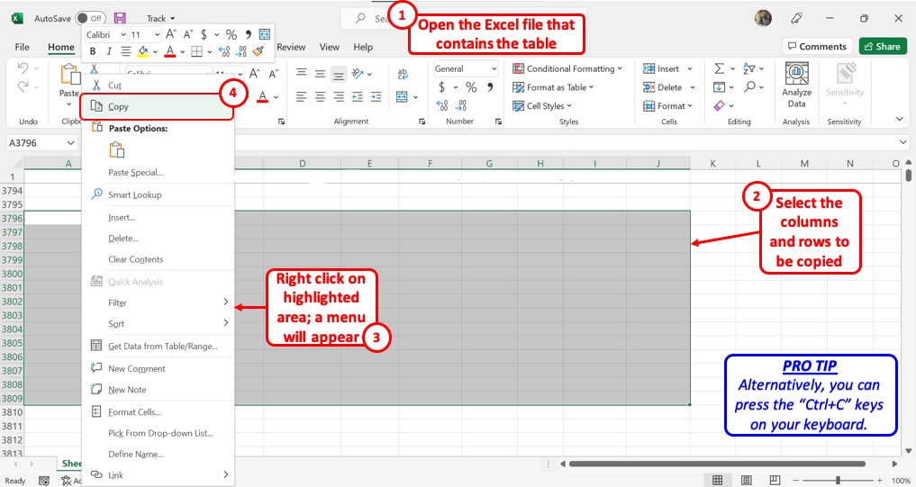
The first step is to open the Microsoft Excel worksheet from where you want to copy the table. Then select the preferred columns and rows to highlight them. “Right Click” on it and click on the “Copy” option. Alternatively, you can press the “Ctrl+C” keys on your keyboard.

Step-2: Click on the “Paste” option

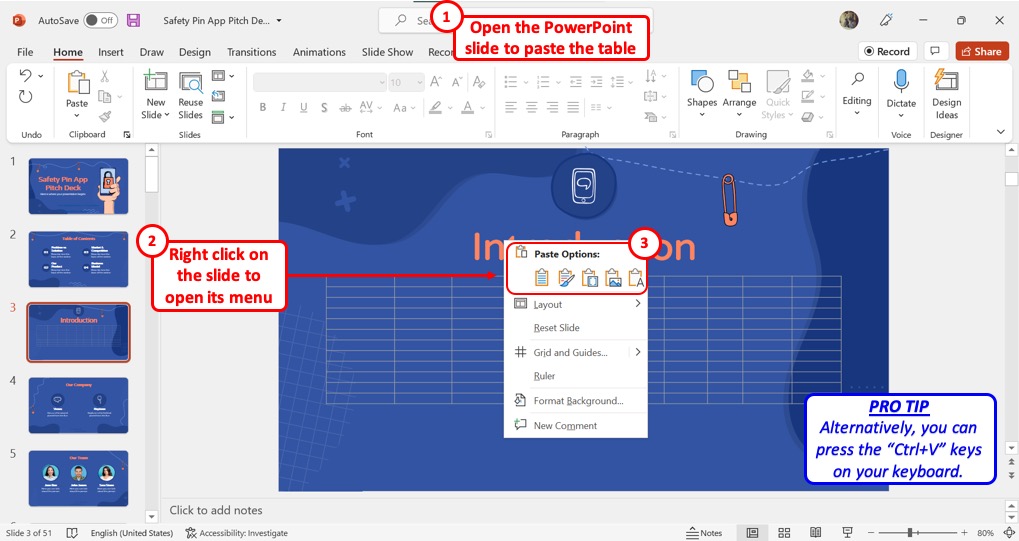
The next step is to “Right Click” on the PowerPoint slide where you want to add the table. In the right-click menu, click on your preferred option under “ Paste Options ” . You can alternatively press the “Ctrl+V” keys on your keyboard to paste the Excel table to your slide.

1.2 Method 2 – Using Paste Special

In Microsoft PowerPoint, the “ Paste Special ” dialog box offers options to paste the copied table in different special formats. To paste the Excel table with a hyperlink, follow these steps.

Step-1: Click on the “Paste Special” option

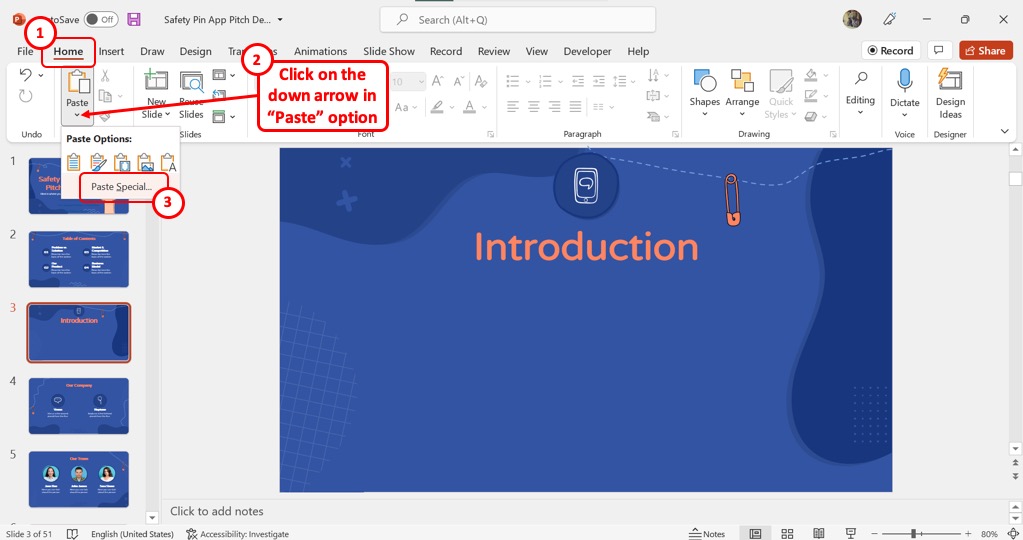
In the “Paste” group of the “Home” tab, click on the down arrow under the “Paste” icon that looks like a clipboard. Then click on the “Paste Special” option from the dropdown menu to launch a dialog.

Step-2: Click on the “Microsoft Excel Worksheet Object” option

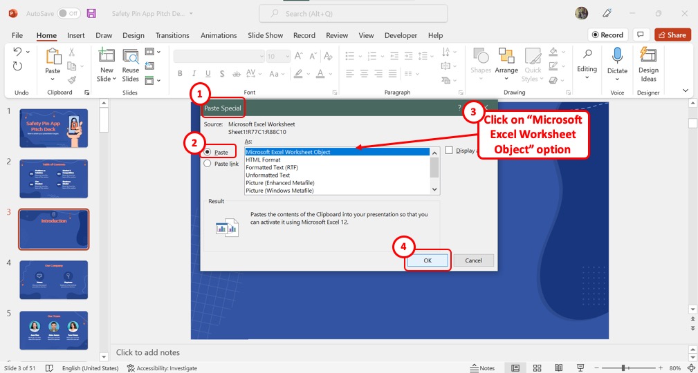
In the “ Paste Special ” dialog box, click on the “Paste” option from the left column. Then in the box in the middle of the dialog box, click on the “Microsoft Excel Worksheet Object” option.

Step-3: Click on the “OK” button Now all you have to do is click on the “OK” button at the bottom of the “Paste Special” dialog box to paste the Excel table in your PowerPoint slide (shown above).

1.3 Method 3 – Using the Insert Object Option (Entire Excel Sheet)

Microsoft PowerPoint also allows you to paste the entire Excel sheet into your presentation slide. For this, you have to use the “ Insert ” tab. Follow the 4 steps below:

Step-1: Click on the “Insert” tab

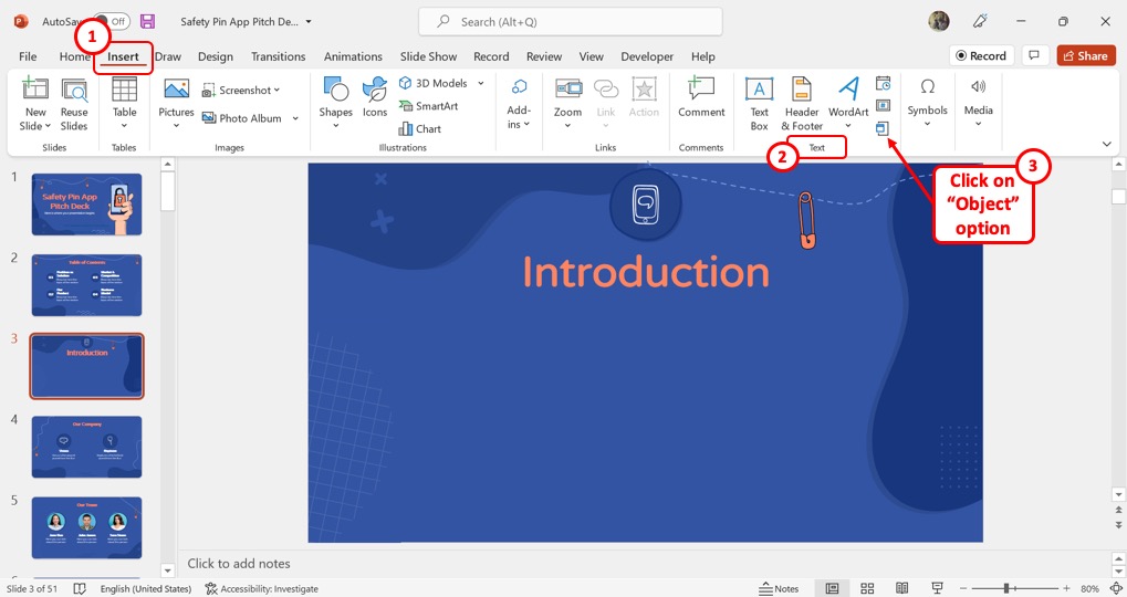
In the menu ribbon located at the top of the screen, click on the “Insert” tab. Under the “Insert” tab, click on the “Object” option which is the last icon in the “Text” group.

Step-2: Click on the “Create File” option

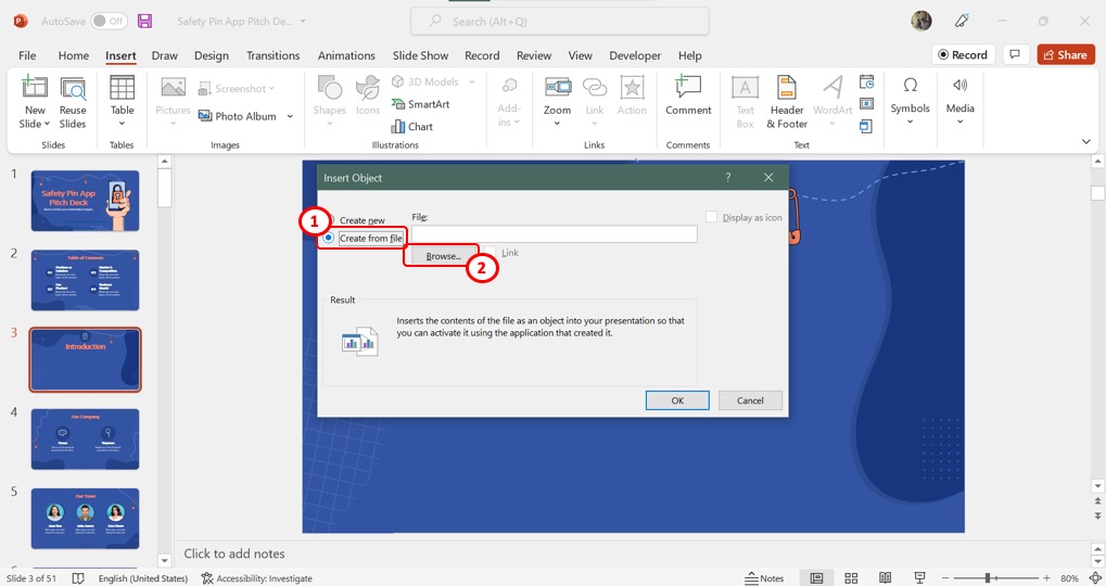
In the left column of the “Insert Object” dialog box, click on the “Create from file” option. Now you can select an Excel sheet to add to the slide.

Step-3: Click on the “Browse” button

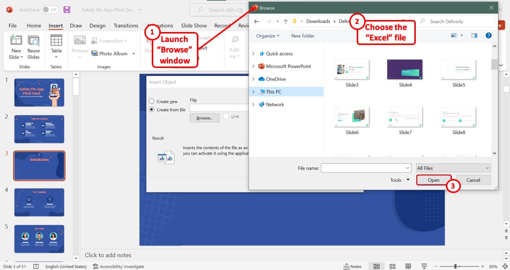
Click on the “Browse” button in the “Insert Object” dialog box to launch the “Browse” window. Select the Excel file and click on the “Open” button at the bottom of the “Browse” window (shown above).

Step-4: Click on the “Link” option

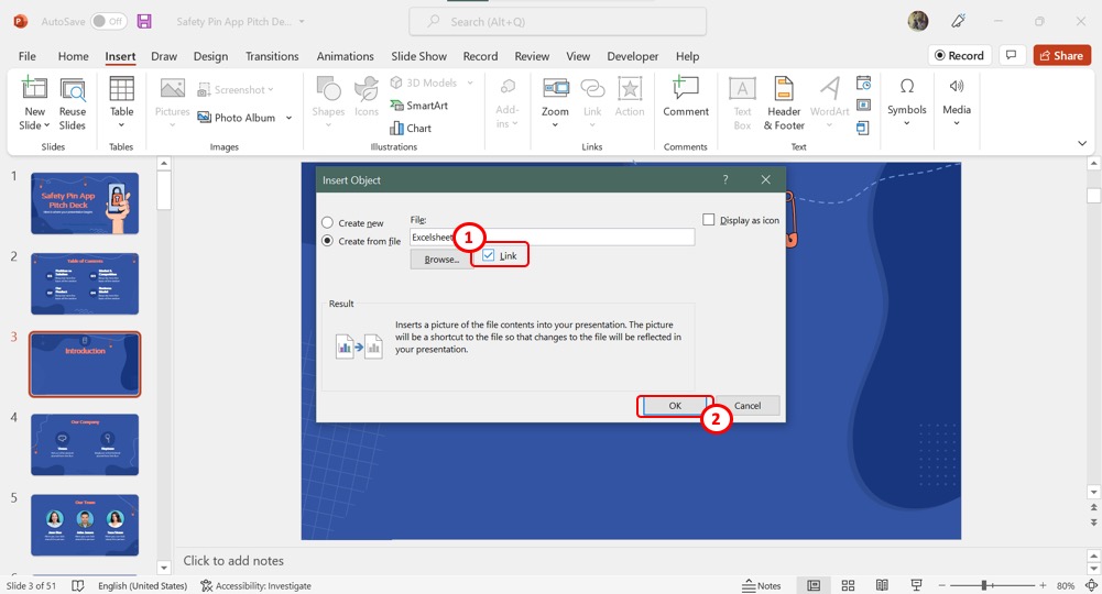
In the “Insert Object” dialog box, click on the “Link” option to hyperlink the Excel table. Click on the “OK” button at the bottom of the dialog box to finish the process.

2. How to Copy Tables from Excel to PowerPoint with Formatting?

When you copy a table from Excel, you can paste it into Microsoft PowerPoint in multiple different formats. For easy editing access, you can use the “Keep Source Formatting” feature.

You can also paste the table as a picture to avoid any accidental edits to the table.

2.1 Method 1 – Using Keep Source Formatting Option

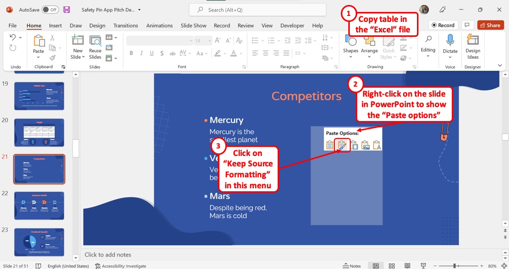
To paste the Excel table as an editable object, you can use the “Keep Source Formatting” option. All you have to do is “Right Click” on the slide and select the “Keep Source Formatting” option under “Paste Options” in the right-click menu. The table in PowerPoint will retain the formatting from Excel.

2.2 Method 2 – Paste as an Image

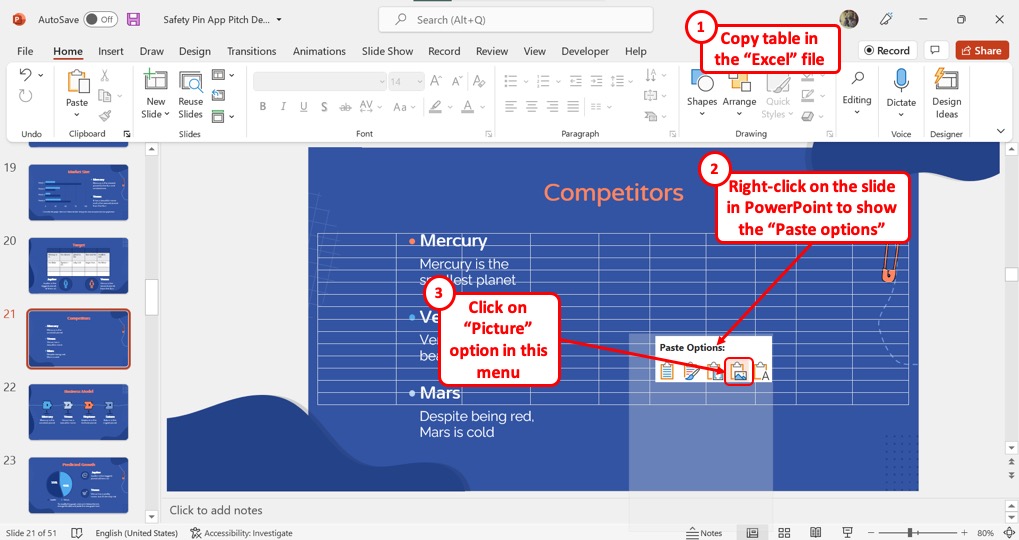
You can paste the Excel table as an image if you do not want any edits to the table. To paste as an image, “Right Click” on the slide and click on the “Picture” option under “Paste Options” in the right-click menu.

3. How to Insert an Excel File into PowerPoint as an Icon?

Instead of pasting a table, you can add an Excel icon in Microsoft PowerPoint. Clicking on the icon during the presentation will lead you to the Excel worksheet. To insert an Excel file as an icon, follow these steps.

Step-1: Copy Table from Excel

Step-2: Click on the “Paste Special” option

In the “ Clipboard ” group of the “Home” tab, click on the down arrow under the “Paste” icon. Then click on the “Paste Special” option from the dropdown menu to launch a dialog.

Step-3: Click on the “Microsoft Excel Worksheet Object” option

Now just click on the “Microsoft Excel Worksheet Object” option in the “Paste Special” dialog box,

Step-4: Click on “Display as icon” The next step is to click on the “Display as icon” option in the right column of the “Paste Special” dialog box. A checkmark will appear beside the option. Now click on the “OK” button at the bottom to insert the Excel file as an icon (shown above).

4. How to Link Existing PowerPoint Table to Excel for Dynamic Data Updates?

In Microsoft PowerPoint 2019 and later versions, you cannot link an Excel worksheet to an existing PowerPoint table. However, any hyperlinked table from Excel in PowerPoint is automatically set for dynamic data updates.

To enable this feature, follow these steps.

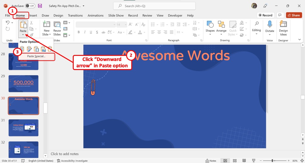
In the “Home” menu, click on the down arrow under the “Paste” icon. Then select the “Paste Special” option from the dropdown menu.

Step-3: Click on “Paste Link”

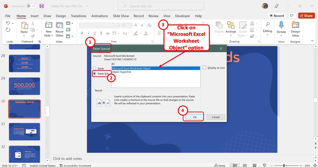
In the left column of the dialog box, click on the “Paste link” option. This will link the table to its Excel source. You can edit the table in either PowerPoint or Excel and find the changes in both files.

Now click on the “Microsoft Excel Worksheet Object” option from the box in the middle of the “Paste Special” dialog box. Then click on the “OK” button to insert the table (as shown above).

5. How to Unlink Table in PowerPoint from Excel?

In PowerPoint, you can remove the hyperlink added to an Excel table. However, you must remove hyperlinks from all objects in the presentation at once. Follow the 2 quick steps.

Step-1: Click on the “File” tab

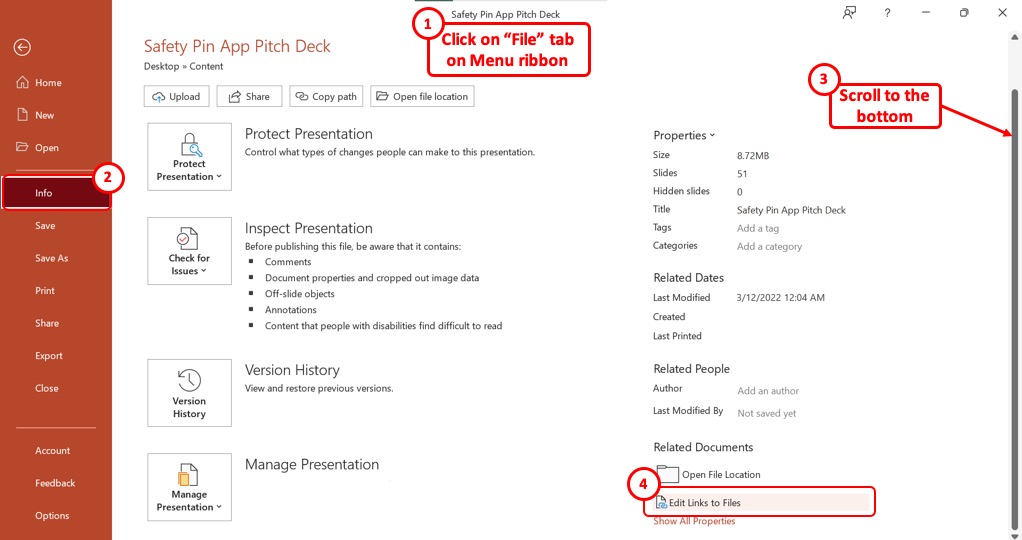
Click on the “File” tab in the menu ribbon located at the top of the screen. In the left sidebar of the “File” menu, click on the “Info” option.

Step-2: Click on “Edit Links to Files”

Now scroll all the way down to the bottom of the “Info” screen. At the right column, click on the “Edit Links to Files” option to remove all the hyperlinks.

6. How to Embed Excel in PowerPoint?

To embed an Excel sheet into a PowerPoint slide, follow these steps.

Step-1: Click on the “Object” option

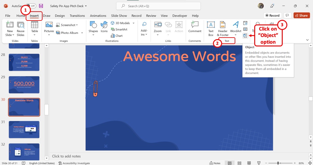
In the menu ribbon located at the top of the screen, click on the “Insert” tab. Then click on the “Object” icon from the “Text” group.

Step-2: Click on “Microsoft Excel Worksheet”

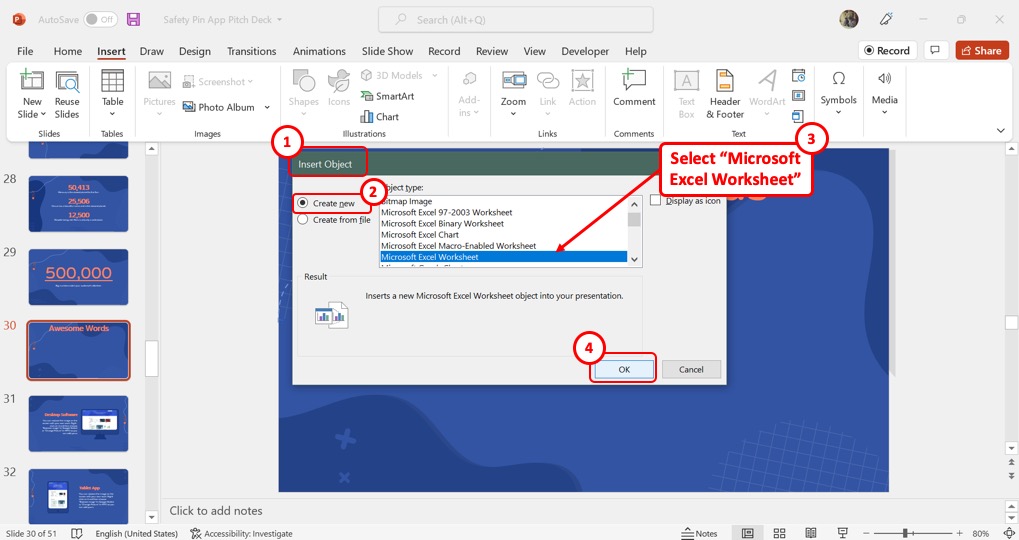
In the “Insert Object” dialog, click on the “Create New” option from the left column. Then select the “Microsoft Excel Worksheet” option from the “Object Type” list. Finally, click on the “OK” button to embed the Excel sheet.

7. How to Insert a Scrollable Table from Excel in PowerPoint?

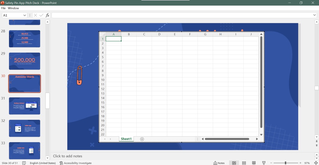
In Microsoft PowerPoint, all the embedded Excel tables are scrollable. To insert a scrollable table from Excel into your PowerPoint presentation, follow the steps discussed in Section 6. However, to make the table scrollable for your viewers, you will need to access the “Developer” tool.

Here’s a link to a Microsoft Support group addressing what you need to do in order to make your table scrollable. Make sure you check that out.

Excel Tutorial: How To Present Data In Excel

Introduction.

Presenting data effectively in Excel is crucial for making informed business decisions and conveying information clearly. In this tutorial, we will cover the importance of presenting data effectively in Excel and provide an overview of the topics that will be covered to help you present your data with clarity and impact.

A. Importance of presenting data effectively in Excel

B. overview of what will be covered in the tutorial, key takeaways.

• Presenting data effectively in Excel is crucial for making informed business decisions and conveying information clearly.
• Understanding the basics of data presentation, such as formatting cells and creating clear tables and charts, is essential.
• Utilizing Excel functions like SUM, AVERAGE, and COUNT, as well as conditional formatting, can help summarize and visually represent data.
• Designing visually appealing charts and graphs and avoiding clutter are important for effective data presentation.
• Using pivot tables for better data analysis and customization can enhance data presentation in Excel.

Understanding the basics of data presentation in Excel

When it comes to presenting data in Excel, it's important to understand the fundamentals of formatting cells and data, as well as creating clear and concise tables and charts. This chapter will cover these key aspects in detail.

Formatting cells and data in Excel is essential for presenting information in a clear and organized manner. Here are some key points to keep in mind:

• Choosing the right data format: It's important to select the appropriate data format for each type of information you are presenting, whether it's numbers, dates, or text.
• Applying cell formatting: Excel offers a wide range of formatting options for cells, including font style, size, color, and alignment. Utilize these features to enhance the visual appeal of your data.
• Using conditional formatting: Conditional formatting allows you to apply specific formatting rules to cells based on their values, making it easier to identify trends and outliers in your data.

Tables and charts are powerful tools for presenting data in a visually appealing and easy-to-understand manner. Here's how to make the most of them:

• Organizing data into tables: Excel's table feature allows you to easily organize and format your data, making it more readable and accessible for your audience.
• Choosing the right chart type: Whether it's a pie chart, bar graph, or line chart, selecting the appropriate chart type for your data is crucial for effective presentation.
• Customizing chart elements: Excel provides a range of options for customizing chart elements such as axes, titles, and legends. Take advantage of these features to tailor your charts to your specific data and audience.

Utilizing Excel functions for data presentation

When presenting data in Excel, it is crucial to use the appropriate functions to summarize and analyze the information effectively. By utilizing functions like SUM , AVERAGE , and COUNT , you can easily generate key insights and draw conclusions from your data. Here's how you can make the most of these functions:

A. Using functions like SUM, AVERAGE, and COUNT to summarize data

• SUM: The SUM function allows you to quickly calculate the total of a range of numbers. Whether you are adding up sales figures, expenses, or any other numerical data, the SUM function provides a simple way to obtain the sum total.
• AVERAGE: When you want to find the average value of a set of numbers, the AVERAGE function comes in handy. This function is particularly useful for determining the average performance, scores, or ratings.
• COUNT: The COUNT function enables you to count the number of cells in a range that contains numbers. This can be helpful for tracking the quantity of certain items, responses, or occurrences within your data.

B. Utilizing conditional formatting for visual representation of data

• Conditional formatting offers an effective way to visually represent your data based on specific conditions or criteria. By applying formatting rules, you can highlight important trends, outliers, or patterns in your data. This can include color-coding cells, adding data bars, or applying icon sets to make the information more visually appealing and easier to interpret.

Designing visually appealing charts and graphs

When it comes to presenting data in Excel, creating visually appealing charts and graphs is essential in effectively communicating your data to your audience. In this chapter, we will explore the importance of choosing the right type of chart for different types of data and customizing colors, labels, and titles for better visualization.

Choosing the right type of chart for different types of data

• Bar charts: Ideal for comparing values across different categories.
• Line charts: Useful for displaying trends over time.
• Pie charts: Suitable for showing the composition of a whole.
• Scatter plots: Helpful in visualizing the relationship between two variables.

Customizing colors, labels, and titles for better visualization

• Color selection: Choose a color scheme that is visually appealing and enhances the understanding of the data.
• Labels and titles: Clearly label each element of the chart and ensure that the title effectively summarizes the data being presented.
• Font size and style: Use appropriate font size and style for labels and titles to improve readability.

Tips for effective data presentation in Excel

When presenting data in Excel, it is important to ensure that the information is clear, concise, and accurate. Here are some tips to help you effectively present data in Excel:

Organize and format the data:

Use charts and graphs:, limit the use of unnecessary details:, set up data validation rules:, highlight erroneous data:, regularly update and review the data:, enhancing data presentation with pivot tables.

Pivot tables are powerful tools in Excel that allow you to analyze and summarize large amounts of data. They can help you present your data in a clear and organized manner, making it easier to identify trends and patterns. In this chapter, we will explore how to create and customize pivot tables to enhance data presentation.

How to create pivot tables for better data analysis

Creating a pivot table in Excel is a straightforward process that can greatly enhance the way you present and analyze your data. Follow these steps to create a pivot table:

• Select your data: Before creating a pivot table, you need to select the data range that you want to analyze.
• Insert a pivot table: Go to the "Insert" tab and click on "PivotTable." This will open a dialog box where you can select the data range for your pivot table.
• Drag and drop fields: Once you have inserted the pivot table, you can drag and drop fields from your data into the Rows, Columns, Values, and Filters areas to customize the layout of your pivot table.
• Summarize your data: Use the "Values" area to summarize your data using functions such as sum, average, count, etc.

Customizing pivot tables for clear presentation of summarized data

After creating a pivot table, you can customize it to present your summarized data in a clear and organized manner. Here are some ways to customize your pivot table:

• Format your pivot table: Excel offers various formatting options to customize the appearance of your pivot table. You can change the font, color, and style to make your pivot table visually appealing.
• Apply filters: Use the filter options in the pivot table to narrow down the data and focus on specific subsets of your data.
• Use slicers: Slicers are visual controls that allow you to filter data in a pivot table. They provide a quick and easy way to analyze and present your data.
• Add calculated fields: If the standard summary functions do not meet your needs, you can create calculated fields to perform custom calculations in your pivot table.

In conclusion, this tutorial has covered the key points of presenting data in Excel, including formatting, creating charts, and using functions to analyze data. Remember to practice these techniques and also explore more advanced features in Excel to take your data presentation skills to the next level. With dedication and exploration, you can become a proficient Excel user and wow your audience with compelling data presentations.

Immediate Download

MAC & PC Compatible

Free Email Support

Related aticles

The Benefits of Excel Dashboards for Data Analysts

Unlock the Power of Real-Time Data Visualization with Excel Dashboards

Unlocking the Potential of Excel's Data Dashboard

Unleashing the Benefits of a Dashboard with Maximum Impact in Excel

Exploring Data Easily and Securely: Essential Features for Excel Dashboards

Unlock the Benefits of Real-Time Dashboard Updates in Excel

Unleashing the Power of Excel Dashboards

Understanding the Benefits and Challenges of Excel Dashboard Design and Development

Leverage Your Data with Excel Dashboards

Crafting the Perfect Dashboard for Excel

An Introduction to Excel Dashboards

How to Create an Effective Excel Dashboard

• Choosing a selection results in a full page refresh.

Unsupported browser

This site was designed for modern browsers and tested with Internet Explorer version 10 and later.

It may not look or work correctly on your browser.

How to Format Your Excel Spreadsheets (Complete Guide)

• Bahasa Indonesia

Think spreadsheets  have to be boring? Guess again. When you learn how to format an Excel spreadsheet, you can bring data and insights to life.

When you focus on your Excel format, it's easier to share your data. Excel table formatting helps your audience analyze and understand a spreadsheet in less time. 

In this tutorial, you'll learn Microsoft Excel spreadsheet formatting to help you style your spreadsheets. I'll use my decade of experience in accounting and finance to give you expert Excel file formats.

• How to Format an Excel Spreadsheet (Watch & Learn)

We've got a helpful video walkthrough for spreadsheet formats. This screencast will teach you how to format an Excel spreadsheet with common techniques.

Read on to find out more about the Excel formatting tools that you can use to change the look and feel of a spreadsheet. We've got an illustrated guide with Excel file format options to make your data digestible.

Jump to content in this section:

Why You Should Apply Excel Sheet Formats

• How to Use Excel Format Options

How to Use Built-in Cell Styles

• How to Achieve Faster Excel Formatting in Excel with Format Painter

How to Turn Off Gridlines in Excel

How to format excel data as a table, how to use conditional formatting in excel, basic ai excel sheet format tools, learn more about microsoft excel, the best source for excel templates (with unlimited downloads), you just learned how to format an excel spreadsheet.

If you're a creative, you might shy away from spreadsheets. Excel is for accountants, right?

Guess again. Spreadsheets are great tools for managing projects, organizing your work, and sharing information with others. And using stylish Excel file formats lets you exercise your creativity!

Formatting Excel spreadsheets isn't just about making them "pretty." It's about using the   built-in styles to add  meaning .   A spreadsheet user should be able to glance at a cell and infer its meaning. 

Above all, your Excel formats should be applied consistently. One example is using yellow shading each time you're making a calculation. This helps the user know that the cell's value will change. Let's learn more about tools for how to format Excel sheets.

How to Use Excel File Format Options

When you're thinking about styling a spreadsheet, it helps to know the tools of the trade. Let's start with the essentials of Excel format options. Here are some of the most popular Excel table formatting tweaks and how you can use them.

The tips in this section were written using Windows and Office 365. If you’ve got a different operating system or a different version of Excel, your steps may be slightly different.

1. How to Use Bold, Italic, and Underline

Bold, italic, and underline are basic Excel format options, but don't underestimate the meaning they can add.

To apply any of these effects, simply highlight the cells that you want to apply the effects to, and then click on the icons on the  Font  section of the  Home  tab.

You probably already know what these three tools do, but how should you use them for Excel file formats? Here are some ideas for how you can apply those styles:

• Bold . Draw attention to key cells using bold formatting. Apply bold to totals, key assumptions, and conclusion cells.
• Italic . I like to use this Excel format style for notes or text that I should de-emphasize. 
• Underline . Add an underline to a summary cell, like a subtotal or conclusion.

In the example below, you can see a simple financial statement for a freelancer before and after I apply basic formatting. These are simple tweaks but dramatically increase the readability.

2. Apply Borders

Borders help to segment your data and wall it off from other sections of data in your spreadsheet. Excel's border tool can apply a variety of borders but can be a bit tricky to get started with. 

Start by highlighting the cells that you want to apply a border to. Then, find the Borders dropdown menu and choose one of the built-in Excel format styles.

Learning how to format an Excel spreadsheet is easier with these pre-built options. As you can see from the dropdown options, there are many options for applying borders. Simply click on one of these border options to apply it to cells.

One of my favorite border styles is the Top and Double Bottom Border style. This is ideal for financial data when you've got a "grand total."

Another option is to change the weight and color of the border. With the bordered cells selected, return to the Borders dropdown menu. You can use the Line Color  and  Line Style  settings to tweak the style of the borders.

Remember to use Excel sheet formats only for your key data. If you emphasize every cell, nothing stands out. Thick borders are ideal for setting a boundary for header columns or the subtotal at the bottom of your data. 

3. Use Shading

Shading, also called fill, is the color that fills a cell. To use this, click and highlight any cells that you want to add shading to.

Then, click the arrow next to the paint bucket dropdown on the  Font  tab on the Home ribbon. You can pick from one of the many color thumbnails to apply it to a cell. I frequently use the More Colors  option to open a full-featured color selection tool. Light shades are best for keeping the text readable.

You can highlight key data using shading. As I mentioned earlier, one idea is to use a consistent fill based on the contents of the cell, such as blue for any "input" fields where you manually type data.

Don't overdo it with shading. When you use too many Excel format options, it distracts from the content that's stored in the spreadsheet.

4. Change Alignment

Alignment refers to the way that the content in a cell is aligned to the edges. You can left align, center, or right align text. By default, content is left aligned in a cell. When you've got  large data sets, you might want to alter the alignment to enhance readability.

One common change that I make is putting text on the left edge of a cell, while numeric amounts should be right-aligned. Also, column headers look great when they're centered along the top.

Change the alignment using the three alignment buttons on the Alignment  tab on Excel's Home ribbon. You can also align content vertically, specifying whether the content aligns to the top, middle, or bottom of the cell.

One of my favorite ways to style a spreadsheet rapidly is to use built-in Excel formats. On the Home  tab, click on the  Cell Styles  dropdown to apply one of the built-in styles to a cell.

Use these pre-built styles to save time. There's no need to rebuild your Excel doc formats from scratch. Use these as a way to take a shortcut to Excel spreadsheet formats.

For even more pre-built Excel file formats, check out the article below. You'll see top options for Excel formats for invoices, with ready-to-use spreadsheet format examples.

How to Achieve Faster Excel Formatting in Excel With Format Painter

Who wants to recreate Excel cell styles over and over again? Instead of recreating the wheel for each cell, you can use the  Format Painter  to pick up formatting and apply it to other cells.

Start by clicking in the cell that has the format that you want to copy. Then, find the Format Painter  tool on the Home tab on Excel's ribbon. Click on the Format Painter , and then click on the cell that you want to apply the same style to.

Don't start from scratch with your Excel file format options! Learn more and master the format painter in the tutorial below:

As you probably already know, a spreadsheet is made up of rows and columns . Rows are ruled by horizontal lines and have numbers next to them. Columns are split with vertical lines and have letters at the top to refer to them.

Where rows and columns meet,  cells  are formed. Cells have names for which row and column they intersect. For example, where row 4 and column B meet is called B4. 

Here's one of my top tips for how to format an Excel spreadsheet for sharing: turn off gridlines. It gives a much cleaner appearance and can be easier to read.

When you're working  in Excel, gridlines are helpful. But when you want to share data , it might be best to turn them off for easier reading. Click on the View  menu, and untick Gridlines. 

Gridlines are imaginary and are only visible on screen. With proper borders added, it's best to turn off gridlines as a finishing step.

How to Print With Gridlines

What if you want to show gridlines throughout the spreadsheet when you print it? Instead of having to manually add borders to each and every cell, you can simply print your workbook and include those gridlines.

To turn on gridlines when printing, start by going to the  File  menu, and choose Print . Then, click on Page  Setup  to open the settings. This controls how your spreadsheet format prints.

On the  Sheet tab, tick the box labeled  Gridlines to include gridlines when you print your Excel workbook.

Keep in mind that this option will certainly use more ink when printing. However, it also might make it easier to read your printed spreadsheet.

One of my favorite ways to style a dataset quickly is to use the  Format as Table  dropdown option. With just a couple of clicks, you can transform a few rows and columns into a structured data table.

When you format data as a table, you unlock many helpful options. For example, you can use the  Table Style Options  section on the ribbon to add automatic subtotals, or use the built-in Table Styles  for quick formatting.

This feature works best when you already have data in a set of rows and columns and want to apply a uniform style. It's a combination of style and functionality, as tables add other features like automatic filtering buttons.

Learn more about why tables are a great feature in the tutorial below:

What if the format of a cell could change based on the data inside it? This feature is built into Excel, and it's called Conditional Formatting.

Imagine using Conditional Formatting to highlight the top and bottom values in your cells. It makes it easy to visually scan your data and look for key indicators.  And don't think that you have to manually adjust it every time your data changes!

Conditional Formatting is best used with numeric data. To get started, simply highlight a column or row of data and make sure that you're on the Home  tab on the ribbon.

There are a number of styles that you can choose from the Conditional Formatting dropdown menu. Each of these applies a different style of Excel formatting to your cells, but each will adapt based on the cells that you've highlighted.

These are just a few tips to help you get started with conditional formatting in Excel. Check out the guide below to learn more about how to apply smart styles to your cells.

Artificial intelligence is a part of more apps than ever. Microsoft Office, including Excel, is no exception. These tools save time during Excel table formatting. In Excel, the Copilot tool can use conversational prompts to apply Excel file format adjustments.

For an AI-powered assist, check out the new Microsoft Copilot Assistant. It can even help you intelligently apply formatting. Learn more below:

The possibilities in Excel are endless. This tool powers companies of all sizes and is flexible for every purpose. But it also features a learning curve that takes time to conquer.

We've got you covered. You've learned how to format Excel spreadsheets effectively. Keep going with more tutorials that help you master Excel:

Need a jumpstart learning how to format Excel sheets? We've got you covered with pre-built templates that have the work done  for you . On Envato , you can download unlimited templates, all in one place.

Think spreadsheets are doomed to be black and white? Now you know that's not the case. You learned how to format Excel sheets with meaning. Each cell's style can help the viewer analyze and understand faster than plaintext alone.

Don't forget that pre-built Excel templates give you great styles with less work. You can even use these styles as inspiration for your own spreadsheets.

Now, it's your turn. Put your new Excel file format options into practice. Open a spreadsheet, add new styles, and watch it come to life!

Contextures Blog

Excel tips and tutorials

PowerPoint Slides From Excel List

If you have a list of names or topics in Excel, here’s how you can quickly create PowerPoint slides from that list. Unlike most of my macros, these run in PowerPoint, to pull the data from Excel. That was easier than writing Excel macros to make things happen in PowerPoint!

Create a Slide for Each Excel Item

In these macros, the main PowerPoint slide is duplicated. Then, the data from Excel is added to the text boxes on the new slide.

There are 4 macros, with variations for

• 1 or 2 text boxes on the slide
• all Excel rows, or based on criteria

You can download the free files from my Contextures site . There’s a zipped folder with the PowerPoint presentation, and an Excel file with data for the slides.

Slide Data in Excel List

There’s a small named table in the sample Excel file, with data for the PowerPoint slides.

You can use this for testing, before trying the macros with your own Excel data.

PowerPoint Main Slide

In PowerPoint, the first slide in the presentation has two text boxes.

The macro duplicates the first slide, and puts the Excel information in those text boxes

In the sample file, don’t move the main slide, if you want the macros to work correctly!

That first slide in the presentation is based on a Master slide.

• You can edit its Master slide, to change the background or text box settings.
• You can also replace that chart icon with your company logo, or add other features.

More PowerPoint Slides

In the PowerPoint file that you can download from my Contextures site, there are 2 other slides.

• Those additional slides have notes on using the macros, and formatting the Slide Master.
• These slides aren’t needed by the macro, and you can delete them.

How to Run Macro to Create Slides

To create PowerPoint slides, from a list in Excel, follow these steps:

• Open the Excel file where your list is stored
• Activate the sheet where the data is stored – the list must be formatted as a named Excel table
• Open the PowerPoint presentation that contains the macros and main slide
• Be sure the main slide, that you want to duplicate, is the first slide in the presentation
• At the top of PowerPoint, on the View tab, click Macros
• Select one of the Create Slides macros, and click Run

Check the New Slides

After the macro runs, you can check the new slides that were added to the PowerPoint presentation.

• In this example, I ran the macro for 2 text boxes, and checked column 3 in the data, for a “Y”
• Three of the rows have a “Y”, so 3 slides were added to the presentation.

NOTE : This macro code is further down the page, and all four macros are in the sample PowerPoint file.

Save the PowerPoint Slides

After you run the macro, and create the duplicate slides:

• Save the PowerPoint file with a new name .
• Then, in that new file, delete the main slide and the two notes slides, or hide them.

NOTE : If you simply export the new slides, you’ll lose the formatting, because they’re based on the Master Slide in the original PowerPoint file.

Create a Presentation Template

Another option is to save the PowerPoint file in PowerPoint Macro-Enabled Template (potm) format.

By default, that file will be saved in your Custom Office Templates folder.

Then, to create a new set of slides from Excel data:

• In PowerPoint, click File, then click New
• In the Templates section, click Personal
• Click on the Slides from Excel template, then click Create

PowerPoint Slides From Excel Macro Code

Here is the code for the CreateSlidesTest_Text2   macro that fills two text boxes on a slide, and checks the Excel table for criteria.

NOTE: To use the macro with a different Excel table, you can change the variable settings, in this section of the macro code.

This macro creates slides for items in the Excel list, after checking a criteria cell, and fills 2 text boxes.

• In Excel, checks the test column ( colTest ), and creates a slide if it contains the specified text string ( strTest )
• In the PowerPoint slide, text from the specified columns ( col01 and col02 ), is entered in the 1st text box and 2nd text box

Learn More About PowerPoint Macros

There are PowerPoint code samples on the Microsoft site , that helped me get started with these macros to create slides from Excel data.

For more examples, you can check the StackOverflow forum, or PowerPoint sites.

Get the PowerPoint Slide Files

The macros that create slides are stored in the PowerPoint file. There are no macros in the Excel workbook

______________________________

PowerPoint Slides from Excel List

_____________________________

4 thoughts on “PowerPoint Slides From Excel List”

Does this work on Macs? I keep getting the “No Excel table found on active sheet” when I try to run it. I’ve been using the sample slides and sample worksheet and I am sure to have the sheet with the table “activated” (clicked on? this just means clicked on, right?) when I try to run the macros. None of them work, they all give the sam error message. I also went into VBA editor Tools/References in both programs to make sure the other was clicked on. No luck. Thoughts? Help?

I don’t think it works on Macbook. I had the same error, tried it on a Windows laptop and worked perfectly.

It also has some problems with large data sets and stops running the code after a few hundred rows, (I had almost 1000 rows) but a quick fix would be to delete the rows that it has already done and run again. It will add the new slides after the last slide in the powerpoint.

To the person behind this: thank you so much. You have saved me hours of my life. I was populating each of my slides manually and it took me the whole day to get through 1/16th fo the work. With this code, took me <5 minutes. Thank you so much.

Did you ever figure out how to do this on a mac? If so, please share…

When I click RUN, it only makes about 10 of 219 slides. I am trying to do a list of names. The error says “Could not complete Slides”

Any help would be appreciated

Leave a Reply Cancel reply

Your email address will not be published. Required fields are marked *

This site uses Akismet to reduce spam. Learn how your comment data is processed .

Introduction Generally, it's not enough to create a model with the spreadsheet. You must be able to present the results to other people; either your boss or your client. This page is dedicated to improving the presentation of the worksheet. Here are some of the options that can be used to improve the presentation of your worksheets. Improving the presentation of your worksheet Often, you will have to present the results of your spreadsheet to many people. There are several possibilities available for improving the presentation. Excel offers you these options in two different ways: by using the Format toolbar or the main menu under the and options.   Format toolbar If you don't see this toolbar in the screen, make the following operations. menu, select the option. . The Format toolbar groups together several possibilities. You can change the font, the size as well put the text in , or . You can align the text or the number in the cell to the left, the middle or to the right side of the cell. You can also align the text on to several columns. This is designed to align a main title over several columns. Write the text that you want to center in the leftmost cell you then make a block with the test that you want centered. Then press on the fourth button for the alignment, that the one with the letter " a " and two horizontal arrows. You can also change the presentation of the numbers in the cells. You can place the monetary format with two decimals, the percentage format, or group together numbers by the thousands. Youcan also add or remove decimals in the presentation. But this is only for presentation purposes. It does not affect the real number in the cell. For example, if the true number of the cell is 12,4 and that you want to present it without a decimal, the number that will appear in the cell will be 12. However Excel will use the "true" value to make any calculations. So, the result of the cell multiplied by 5 will not be 60 (5 * 12) but really 62 (5 * 12,4). You can also change the presentation of the cell itself. You can frame the cell or a group of cells, with various types of rows. Change the background color and the pattern of the cell. With the last option of the toolbar, you can modify the color of the text. This can bo done for one letter or the entire content of a cell. Format of the cell There are other ways of changing the presentation of your file. In the main menu under the menu and options, you will find the options available to modify the presentation, including others that are not in the Format toolbar. You will find the options under the following six tabs. menu, select the option. tab. In this window, there are six tabs that offer all the possibilities for cell presentation. As you can see, there are a lot more options available from the toolbar. Under the first tab you will find the options to change the presentation of numbers. In the categories box, there are several styles of presentation for numbers and text. You can even personalize the presentation according to your needs. In the right part of the window, you have options according to the style of presentation that you chose. In the picture on the left side, you can determine the number of decimals that will be shown, the monetary symbol and the color of the number if it's negative. You can even personalize the numbers according to your needs. From this window, you can adjust the text within a cell. You can paste the text horizontally to the left or right side of the cell's border. You can adjust the vertical position of the text within the cell by changing the position to the bottom or to the middle of the text. One of the new options allows you to change the orientation of the text. You can also give an angle to your text! This is interesting for titles and some descriptions. However do not exaggerate its use. From this window, it's also possible, to merge or demerge cells. To merge you must first make a block with the cells to merge you want merged. Then go to the window to the left in order to activate the " " option. To remove the fusion, deselect the last option. From this window, you can modify the characters of the cells. You can also change the font, the style, the size, the background and the color of the text. From this window, you can determine the outline of a cell or a range of cells. You can choose the style of the row (none, simple, double, thick...) and the color of your choice of the right-hand side of the window. From the left-hand side, you can chose the place you want the row to appear by pressing on one of the buttons surrounding the outline. You can also click inside the outline to fix the rows. Excel offers you also the possibility of modifying the color of the cells and even adding a pattern to it. Always verify that the text remains visible when chosing a patern. . This tab is very practical when you want to protect a workfile. It prevents other users from modifying formulas but still permits them to view and use the worksheet. The Excel protection option will protect all your worksheets. The protection tab allows you to lock or unlock cells within the worksheet. The protection is made in two stages. You must indicate to Excel the cells that you want . It's these cells that the users will be allowed to change. All other cells will be locked and cannot be changed. The second stage consists in protecting the worksheet or all the spreadsheet. When you'll have to unprotect the appropriate cells: Excel offers you the choice to protect the worksheet, the spreadsheet (the file) or to be able to share the document with the other people. You can determine the elements of the sheet that you want to be protected. You can also put in a password to protect the worksheet or the file. It's however not compulsory. You can leave the empty box and the sheet will be always protected until somebody removes the protection. Do not worry if you put the protection and forget the password. There are software or macro for Excel that exists "to crack" the password. It's going to take only a few seconds to discover and remove it. To find these software, use a research site and look for the words crack or password and excel. You cannot "crack" a password of a document without having first the permission from the owner of the file. Otherwise, you're in big trouble!!! As soon as you go to try to change a value, Excel will present you the message above. The software warns you that this worksheet is protected and that you cannot change the contents of protected cells. For the moment, remove the protection on the worksheet. Copy a formatting style It's first necessary, to apply a presentation style to a cell. It's now necessary to copy this format of presentation to the other cells of the example. It's the format of presentation of this cell that will be copied on the others. The designers of Excel found an easy method to apply the same presentation style to several blocks. The next exercise consists of applying a presentation style to several separate cells. You now see how easy it's to quickly prepare a presentation for your spreadsheet. There is an even faster way: the automatic format. You can spend a lot of time trying to improve the presentation of a file. Excel offers you, predefined formats for presentation. It's enough to apply the presentation style of your choice to the area of cells that you want. This is what you're data would be like when using one of the formats available. It took only a moment. Conditional format The conditional format allows you to change the presentation only when a series of events apply. For the example below, you want the quantity available to appear in red when the is lower than the minimal quantity. The change in colour allowes you to notice more rapidly when your inventory is too low. Note: To be able to enter several rows of text in the same cell, you must use the Alt and Enter keys. Y ou must now write a condition and choose the kind of presentation when this condition occurs. The second box determines the kind of condition. As you notice it's a very complete list. For this condition, you want to compare it with the contents of the B2 cell. It's also possible to add up to 3 conditions and to change the presentation under different circumstances. You just need to press the Add button to add another condition. For the moment, there are no need for another condition. The conditional format is placed in the A2 cell. It's time to test it. Here is the result. The number is now in red. This happens only when the number of this cell is lower than the minimal quantity declared in B2 cell . You can add conditions or remove them. Experiment with different numbers and think where you could apply this option in your models. Newly Launched - AI Presentation Maker Researched by Consultants from Top-Tier Management Companies AI PPT Maker Powerpoint Templates Icon Bundle Kpi Dashboard Professional Business Plans Swot Analysis Gantt Chart Business Proposal Marketing Plan Project Management Business Case Business Model Cyber Security Business PPT Digital Marketing Digital Transformation Human Resources Product Management Artificial Intelligence Company Profile Acknowledgement PPT PPT Presentation Reports Brochures One Page Pitch Interview PPT All Categories Top 30 Excel Linked Data-Driven PowerPoint Slides and Templates Gunjan Gupta It’s time to dump spreadsheets and move to waterfalls or even donuts for that matter to show your data in ways that people absolutely adore! Have you ever noticed that people often groan when a spreadsheet pops up in front of them sharing brilliant data insights? No matter how useful the insights are, the reaction isn’t what a presenter wants. Rather it is far away from his imagination. Maybe it’s not the audience- or the presenter- to blame. Maybe it is the old school method that is the real culprit. Or maybe the presenter suffers from Dumb-and-Overused-Chart-Syndrome ? Haven’t heard of this syndrome before? Unfortunately without even realizing, many presenters are suffering from this so-called syndrome wherein the charts and graphs aren’t engaging enough, thus yielding a negative reaction from the audience- groans, yawns-all at once! Here are 30 excel linked data-driven PowerPoint slides and templates that can help in presenting data in a clever way and up your data visualization game. These charts don’t require the audience to squint; instead, they act as data visualizations tools and do the same that a photo does to everything else: Show not tell! So, now you can stop boring your audience with the same old-school spreadsheets and try serving them some Donuts, Waterfall, Bubbles , so on and so forth.  Trust me it is more fun, and if you are still not convinced. Try it for yourself! P.S- All these charts are data-driven and excel-linked, taking your presenting game a notch higher.  Tornado Chart For Population Excel Chart Template 1 The core of every business’s success lies in properly analyzing the data and using it to one’s advantage. Each high-quality presentation should show reliable research and analysis. We have designed this tornado chart to help you illustrate trends more easily and show important relationships between the population of males and females in a country or workplace. This diagram is a uniquely designed bar chart that performs sensitivity analysis, thus making it ideal to be presented in front of anybody depending upon your needs and requirements. Since this, a data-driven Excel linked chart you will face no difficulty in tailoring it to your current preferences.  Download Tornado Chart For Population Pyramid Excel Chart PowerPoint Layout Global Market Statistics Pie Chart With Percentage Template 2 Visualize and compare various proportions of categories with this pie chart template. Divide categories into segments showing how individual components contribute to the total. This is an effective data visualization chart that can be used to process data efficiently. You can show various combinations of numerical data with this template that is data-driven, thus making editing and adding your personalized data a breeze. Besides this, it is the most compatible set to present a small amount of data that can be easily comprehended by the viewer.  Download Global Market Statistics Pie Chart With Percentage PowerPoint Slides Company Net Promoter Score Template 3 Analyze customer satisfaction and promotional score with this template. This template is great for sales and marketing professionals looking for effective ways to explain the NPS in a seamless manner. This template has a diverse collection of data-driven chart illustrations that can help in depicting various components of NPS like the total number of respondents, active users, passive users, and others. Not only this, but it can also be used to present any information, visually that can be easily altered to fit your needs and requirements. Simply add your preferable data and edit this template on the go.  Download Company Net Promoter Score Survey Analysis PPT Slide Globe With Bar Graph Data-Driven Success Template 4 It doesn’t matter if you're an HR executive, manager, entrepreneur of any other individual this chart template can be used by anybody time and again to present complex data. The data presented using this chart is very easily understandable and can be retained by the audience for a long period of time, hence individuals belonging to any sector can benefit from this template. Besides this, it is great to present demographic information with ease as it is a fully editable layout. Its data-driven quality gives you enough scope to add your personalized data and present it in a seamless manner.  Download Globe With Bar Graph Data Driven Success Indication PowerPoint Slides Data Comparison Chart Template 5 Compare and visualize two sets of data with this template. Use it to show a comparison between products, gender, etc. The applications of this template are multiple hence it can be used to visualize all forms of data comparisons. Presented in the form of vertical and horizontal bar graphs this template provides a clear view of the comparison, thus making the judgment regarding the aspects very easy for the user and viewer as well.  Download Data Comparison Chart PowerPoint Slide Speedometer With Three Text Boxes Template 6 This is a fully editable speedometer design that can be incorporated in any of your dashboards or used individually to present data in a seamless manner. It functions well in business presentations as it is easily comprehended by the audience. You can use it to indicate the performance level, tasks completed, reporting the status of the project, etc. The set is completely user friendly and made with high-resolution images that make the presentation of KPI’s very easy and convenient for the user.  Download Speedometer With Three Text Boxes PowerPoint Slides Data-Driven Human Resource Management Template 7 This is a very creative template that can be used to show any data analysis depending upon the needs and requirements of the user. It is also a data-driven chart, hence you will face no difficulty in adapting it to any data analysis whether it is related to any field business, marketing, sales, or any other. It all depends on the requirements of the user which is efficiently fulfilled with this colorful template. Data-Driven Pie Chart And Donuts For Analysis Template 8 This template is apt to present an analysis of demographic spread, global market, economic factors, and others. The chart uses a minimalist approach making it visually appealing and comprehensive. It is also a well-accepted layout in the business field to report, show percentage reviews, market share analysis, etc. Users can make use of this template to show a multitude of statistics depending upon the needs and requirements of their business. Built with user focus friendliness, this template can be used to present quality presentations to the audience.  Download Data Driven Pie Chart And Donuts For Analysis PowerPoint Slides Waterfall Chart Showing Sales Goal Variance Template 9 This waterfall chart template is useful to get a quick overview of sales goals of your organization. It can be used to show both positive and negative values over a period of time. It can also be used to point out the initial and end values of the sales goals that can be altered as per one’s needs and requirements. Since this is a data-driven chart you will face no difficulty in modifying the data as per your presentation demands.  Download Waterfall Chart Showing Sales Goal Variance Self Presentation Visual Resume PPT Template 10 Are you applying for a new job position wherein you need to stand out from the rest of the candidates? Make use of this visual resume template with data-driven charts and graphs, that offer a unique way of presenting your abilities, skills, qualifications, previous employment history, and other aspects of your personality. These charts and graphs provide an at-a-glance view of the jobseeker’s qualities, thus helping them get noticed. Also, this template is designed to fit your creative aesthetic style by using professional colors and high-quality images making it easily shareable.  Download Self Presentation Visual Resume PPT Template Self Presentation Resume Format Template 11 Want a resume that leaves an everlasting impression on the employer? This set comes in handy with its data-driven content and other attributes. It comes in a uniquely designed, clean infographic layout that offers a host of benefits to the job seeker in terms of bagging great employment opportunities. Its automatic updation quality helps the user to present his preferred data in a pleasing manner, thus helping his job application stand out from the rest. This template is Excel linked so sharing it and editing it is very easy and convenient.  Download Self Presentation Resume Format Editable PPT Slide Risk Management KPI Dashboard Template 12 Risk management is the most crucial vertical to mitigate risks. This risk management kpi dashboard template acts as a resourceful tool that can be used to identify, monitor, and minimize various kinds of risks as it provides useful information in the form of a snapshot. As such anybody can easily understand the trends of risk mitigation, thus making this design an ideal set. Professionals belonging to any sector can use this template to provide all sorts of information about adverse conditions, unforeseen events, and others that are to be measured and monitored continuously.  Download Risk Management KPI Dashboard Showing Consequence Vs Likelihood Data-Driven 3D Interactive Bubble Chart Template 13 Uplift the overall aesthetic appeal of your boring slideshows with this bubble chart template. Present any form of data that you wish to with this data-driven chart that responds to every need of the user. Since this chart offers a wide range of applications it can be used by any professional to represent complex data in an easily understandable manner. Also, the data presented with this template can be easily retained by the audience making it beneficial for any individual downloading it.  Download Data-Driven 3D Interactive Bubble Chart PowerPoint slides 4 Quarters Track Record Template 14 Show various combinations of data analysis with this template. It can be used by HR, entrepreneurs, executives, team leaders or any other person to showcase data in a visually attractive way. Employ this chart to show quarterly track records of sales, marketing, or any other department. This is not a topic-specific template, hence any sector can benefit from it. Also, its data-driven quality enhances its versatility and flexibility as well.   Download 4 Quarters Track Record PPT Ideas Key Performance Indicators Template 15 KPI’s are crucial to measuring the success of a project, tasks,  organization etc. over a given period of time. You can use this template to measure the performance of your organization. Use it to analyze and measure various performance parameters with a single layout. Featuring all kinds of data-driven charts and graphs this template makes viewing the overall performance of the organization very easy and convenient. Hence, it can be used by project managers, strategists, or any other person. All you have to do is download this design, add your data, and see the charts getting altered.  Download Key Performance Indicators Template PowerPoint Slide Show Project Name Status Planning Dashboards Template 16 This project dashboard is ideal for departments or executives to monitor the status of the campaigns, number of projects completed, number of projects planned, their cost, and similar other details. It also contributes to making the organization more intelligent towards attaining its goal as everything can be viewed at a single glance. Besides this, share important information or metrics with this template as it is easily comprehensible making it useful for business owners, project managers, team leaders, and others. It is data-driven which makes it easy to alter and create a well-prepared slideshow in no time.  Download Project Name Status Planning Cost Portfolio Dashboards Workforce KPI Dashboard Template 17 This template is apt to keep a headcount of your workforce whether they are males or females. Keep track of everything pertaining to the employees such as when they started or left the organization, promotions given, grade-wise headcount, etc. This is a dashboard template showing various forms of data-driven charts that function as great visualization tools. As such everything related to the employees can be monitored at a glance, with this template. Besides this, it functions well for every organization because of its versatility.  Download Workforce KPI Dashboard Showing Starters Headcount Leavers Promotions And Joiners Website Performance Review Template 18 Monitor website performance by tracking important metrics like online transactions, traffic source, site consumption time, and others. This is an important tool to collect, measure, and analyze data for your website that is data-driven. Hence, it will get automatically updated as soon as you add your data to it. This template can be used in many different contexts like social media marketing, digital marketing, SEO, eCommerce, and others. Since it provides a broad spectrum view of website KPI’s it will be useful for any organization or agency no matter how small or big it is.  Download Website Performance Review PPT Slide Template Achieving Sales Target Sales Performance And Sales KPI Dashboard Template 19 Measure sales KPIs with a birds-eye view using this template. This template can be used to view key sales indicators to achieve organizational goals more efficiently. This includes metrics like weekly sales, product inventory, net sales, and many others that can be modified as per the liking of the user. Besides this data collected from various sources can be presented with this template to generate actionable insights at a much faster rate.  Download Achieving Sales Target Sales Performance And Sales KPI Dashboard PPT Icon Data-Driven Sales KPI Dashboard Template 20 Executives who want an at-a-glance view of the sales will appreciate this professionally designed template. Showcase various sale scenarios and their corresponding data such as monthly sales, sales volume, through monthly sales comparison and others. This template provides insights into critical sales material without cluttering up the layout. Also, each chart in this template is Excel linked hence you will face no difficulty in altering the data as per your needs and requirements.  Download Data-Driven Sales KPI Dashboard For Achieving Sales Target PPT Samples Financial Performance KPI Dashboard Template 21 This is a high-level snapshot of the financial health of your company that will help you in making responsible decisions. Use it to decide about the various resources and their proper allocation so that they prove advantageous for the company and its finances. This template covers various aspects of financial performance such as vendor expenses, payroll headcount ratio, fundraiser expenses, sales conversions and others that can be easily altered as per one’s liking. It summarizes and interprets the numbers in a very easy format that can be easily understood by the people viewing it, thus making it a highly resourceful data visualization tool.  Download Financial Performance KPI Dashboard Project Status KPI Dashboard Template 22 This is a data-driven project status template that displays important statistics, metrics, data, and other aspects related to the health of the project. It provides a mix of various KPIs related to the project thus enhancing the overall decision-making ability of the project managers, executives, or any other individual who downloads this template. Besides this, it is a user-friendly layout that includes high-resolution charts and graphs that can be altered as per one’s desire.  Download Project Status KPI Dashboard Showing Delivery Roadmap And Resource Allocation Workforce At A Glance PowerPoint Slide Template 23 This is a very widely used tool that helps in visualizing relevant Key Performance Indicators related to HR functions.  Key performance metrics and data such as part-time staff, full-time staff, male-female ratio of the employees, etc. can be efficiently displayed with easy to understand charts and graphs used in this layout. This is a ready-made template that is 100% customizable, owing to the feature of being Excel linked. Download Workforce At A Glance PowerPoint Slide Graphics Procurement KPI Dashboard Template 24 This dashboard helps in keeping track of all the procuring activities with relevant and measurable metrics such as total spend profile by region, total spend profile by operation, top vendors, and many more. It provides a benchmark that can be used to analyze the quality of the warehouse and vendor from which the material has been procured. Numerous KPI’s can easily be viewed with this data-driven dashboard. All the charts and graphs used in this dashboard can be edited as per your data requirements as they are Excel linked, thus making them highly adaptable.  Download Procurement KPI Dashboard Total Spend Analysis PPT Samples Human Resources KPI Dashboard Template 25 This is an advanced analytics tool that can be used to display important HR metrics like recruitment funnel, active pipeline, allocation sources, and many others. It provides an at-a-glance view of the important metrics to the HR department, thus helping them improve the recruiting process, optimize their work, and enhance the overall well-being and performance of the employees. With so many data visualizations that are Excel linked, this template can be adopted by any user as per his needs and requirements.  Download Human Resources KPI Dashboard Showing Recruitment Funnel Application Sources Project Status KPI Dashboard Template 26 Project managers rarely have time to go through multiple spreadsheets to understand how well the project is progressing. The objective of this project status dashboard template is to quickly summarize various aspects of the project’s health such as task status, pending projects, completed products, etc. so that important facts can be presented at a glance. It presents a scannable view of the project, that can be used by any departmental head as per his needs and requirements. The data-driven quality of this template makes it a highly resourceful one to be used for viewing the success and failure of your projects.  Download Project Status KPI Dashboard Showing Project Timeline And Budget KPI Dashboard Template 27 Human Resources is one of the key fundamentals of running a company successfully. This template provides a snapshot of HR metrics such as gender diversity, the average time for new hire, vacation days, and others. Use it to report the important KPIs to executives, managers, and others. Further, it can be used to make viable HR strategies that will prove beneficial for the company as well as employees.  Download KPI Dashboard Showing Overtime Cost Gender Diversity Ratio Three Key Metrics With Business Development KPIs Template 28 Employ this reporting tool to display a summary of business development KPIs and metrics like lost work, new business, amongst others. This dashboard helps in condensing large amounts of data into a single visual representation, thus making it far more comprehensible. Also, its data-driven feature makes it easily adaptable and versatile for any user.  Download Three Key Metrics With Business Development KPIs And Proposal Success Risk Management KPI Dashboard Template 29 Determine and mitigate risks from various verticals with this dashboard template. Use it to examine various adverse conditions and unforeseen events that may lead to various risks. Since the topic of risk mitigation is very diverse, this dashboard template can be used to provide at a glance view of risk analysis, its identification, mitigation strategies, and others with various data-driven charts and graphs. This will surely save your time in creating a dashboard from the very scratch.  Download Risk Management KPI Dashboard Showing Risk Distribution By Country Office And Business Process Financial Ratio KPI Dashboard Template 30 This financial ratio dashboard provides an instant visual representation of the company’s financial health. The finance department can use this layout to track the company’s expenses, profit, loss, revenue, return on equity, etc. in real-time. This helps in identifying the areas that require immediate attention to improve the financial condition of the organization. This template will also help in saving the time and resources of the company as everything is pre-designed and data-driven. All you have to do is download the template, add your data and see the charts getting automatically updated.  Download Financial Ratio KPI Dashboard Showing Revenue Net Profit Margin And Debt To Equity These are our top 30 data-driven charts and graphs and we hope you found them inspiring enough to create your own designs.  Drop your thoughts in the comment section below and download these designs for further motivation! Related posts: Top 10 Metrics, Key Performance Indicators, and Dashboards Google Slides Templates For Business [Updated 2023] Top 35 KPI-Dashboard Templates For Performance Tracking Top 40 Metrics, Key Performance Indicators and Dashboard PPT Templates for Every Business 40 Best Lego Blocks PowerPoint Templates To Unlock Your Hidden Talent Liked this blog? Please recommend us Data Sucks, Says Who? 16 Creative Data Visualization Techniques to Showcase Your Numbers Tweak it to Work it! 10 Golden Rules For Data Visualization How to Turn Ugly Charts That Make No Sense Into Simple, Clean Visual Stories [Updated 2023] 30 Best Gantt Chart PowerPoint Templates For an Effective Visualization of Your Project This form is protected by reCAPTCHA - the Google Privacy Policy and Terms of Service apply. --> Digital revolution powerpoint presentation slides --> Sales funnel results presentation layouts --> 3d men joinning circular jigsaw puzzles ppt graphics icons --> Business Strategic Planning Template For Organizations Powerpoint Presentation Slides --> Future plan powerpoint template slide --> Project Management Team Powerpoint Presentation Slides --> Brand marketing powerpoint presentation slides --> Launching a new service powerpoint presentation with slides go to market --> Agenda powerpoint slide show --> Four key metrics donut chart with percentage --> Engineering and technology ppt inspiration example introduction continuous process improvement --> Meet our team representing in circular format Formatting Worksheet in Excel: 11 Examples 1. Turning Off Gridline in an Excel Worksheet Go to the View tab. The gridlines will turn off from the worksheet. Method 2 – Formatting Title in Excel Worksheet 2.1 using merge & center command. To apply the Merge & Center feature to format the title, apply the following steps: Select the row of the title. We selected the range B2:G2 . This will merge all the selected cells and bring the title to the center of the merged cell. 2.2 Using Center Across Selection Option Merging cells often creates problems in formula-based operations in Excel. To avoid such issues, you can use the Center Across Selection option as an alternative. This option only displays the value as center-aligned. But the value is stored in a single cell only. To format the title with the Center Across Selection option, follow the steps below: Go to the Alignment tab. Set the Horizontal Text Alignment to the Center Across Selection option. This will display the title center-aligned to the row. You can notice that the title value is in a single cell (cell B2 in this case). Method 3 – Applying Cell Borders in an Excel Worksheet 3.1 apply thick bottom border to title. The Thick Bottom Border option is useful for differentiating between sections. Thus, applying this border to the title will visually separate it from the data table. To apply the Thick Bottom Border option in the title, follow the steps below: Select the row where the title is displayed. Click the Borders dropdown from the Font group. There is a thick bottom border in the title row. 3.2 Apply All Borders Command Select the data table. We selected the range B4:G15 . The borders have appeared around each cell of the data table. 3.3 Change Border Color Select the row with the title where the thick bottom border was applied. Click the Borders dropdown > Line Color > your preferred color. Dot  symbols will appear at each corner of cells throughout the worksheet. Click the Borders dropdown again and select the Thick Bottom Border option. Method 4 – Applying Cell Shading in an Excel Worksheet Select the row with the title. Click the Fill Color dropdown from the Font group. Select the range with column headers. We selected the range B4:G4 . As a result, the title and column header rows will have a fill color like the following image. Using similar steps, you can apply cell shading to any range in a worksheet. Method 5 – Changing Font Color in Excel Select the row with column headers. Click the Font Color dropdown from the Font group. The font color of the column headers row has changed to White. Method 6 – Changing Font in Excel 6.1 change font size. Select the range with the title. 6.2 Change Font Style Press and hold the Ctrl key while selecting the title range and column headers range (i.e. range B2:G2 and B4:G4 ). Click the Select All button from the top-left corner of the worksheet. The font in the worksheet has changed now. Method 7 – Changing Data Alignment in Excel Select the data table (i.e. range B4:G15 ). Select the column headers (i.e. range B4:G4 ). The data alignment in your worksheet has changed now. Method 8 – Changing Number Format in Excel 8.1 modify date format. Select the column with dates. We selected the range F5:F15 . Go to the Number tab. Select Date from Category . Choose your desired data format. We selected the dd mmmm yyyy format. The selected date format has appeared in the target column. You may notice ### symbols in some cells due to inadequate column width. We will discuss the process to fix this issue in the upcoming sections. 8.2 Apply Accounting Format Select the column with price values. We selected the range G5:G15 . Method 9 – Changing Column Width in Excel Sometimes you may ### symbols instead of actual values in some cells. It usually happens due to insufficient column widths. To fix this problem, you have to adjust the column width in Excel. You can use the following 3 methods to adjust column width in Excel: 9.1 Use Mouse to Change Column Width Hover the mouse pointer at the column bar’s right side in the desired column. The drag icon will appear. The column width is adjusted, and the dates appear. 9.2 AutoFit Column Hover the mouse pointer at the column bar’s right side in the desired column. The column width will adjust automatically to fit the data in the column. 9.3 Set Column Width to a Specific Number Select the desired column by clicking on the column bar. Right-click on your mouse to open the context menu. This will adjust the column width in your selected column. Method 10 – Changing Row Height in Excel When you add multi-line texts with the Wrap Text feature, the entire data may not be displayed due to insufficient row height. To fix that, you can adjust row heights in your worksheet. You may adjust the row height to adjust the vertical spacing in a row as well simply. Method 11 – Applying Conditional Formatting in Excel Select the rows for which you want to set alternative row colors. We selected the range B5:G15 . Select the rule type Use a formula to determine which cells to format . Set the formatting rule to: =MOD(ROW(B5),2)=0 Click the Format button. Go to the Fill tab. Select your preferred background color. The alternative row colors are applied to the selected range in the worksheet. Download Practice Workbook Frequently Asked Questions How do i quickly change the format of a worksheet. Here are the steps to change the format of a worksheet quickly: Go to the Page Layout tab. Click the Themes dropdown. Hover the mouse pointer over various themes to see the change in the worksheet format. Select your preferred theme. Can I copy formatting from one worksheet to another? Yes, you can copy any worksheet format to other worksheets. Here are the steps to copy worksheet formatting to other sheets: Select the cell or range whose formatting you want to copy. Press the Ctrl+C keys to copy the cell. Go to the target worksheet. Select the cell or range where you want to paste the formatting. Right-click on the mouse to open the context menu. Select Formatting from the Paste Options . How to freeze a row in a worksheet? While working with worksheets containing a large dataset, we often need to freeze rows to keep specific rows visible when we scroll down. Consider a situation where you need to freeze the 5th row in a worksheet. Here are the steps to freeze that row: Click the row bar of the 6th row. From the Freeze Panes dropdown, click the Freeze Panes option. << Go Back to Learn Excel What is ExcelDemy? Tags: Learn Excel Seemanto Saha graduated in Industrial and Production Engineering from Bangladesh University of Engineering and Technology. He has been with ExcelDemy for a year, where he wrote 40+ articles and reviewed 50+ articles. He has also worked on the ExcelDemy Forum and solved 50+ user problems. Currently, he is working as a team leader for ExcelDemy. His role is to guide his team to write reader-friendly content. His interests are Advanced Excel, Data Analysis, Charts & Dashboards, Power Query,... Read Full Bio Leave a reply Cancel reply ExcelDemy is a place where you can learn Excel, and get solutions to your Excel & Excel VBA-related problems, Data Analysis with Excel, etc. We provide tips, how to guide, provide online training, and also provide Excel solutions to your business problems. Contact  |  Privacy Policy  |  TOS User Reviews List of Services Service Pricing Create Basic Excel Pivot Tables Excel Formulas and Functions Excel Charts and SmartArt Graphics Advanced Excel Training Data Analysis Excel for Beginners Advanced Excel Exercises with Solutions PDF Keyboard shortcuts in Excel Many users find that using an external keyboard with keyboard shortcuts for Excel helps them work more efficiently. For users with mobility or vision disabilities, keyboard shortcuts can be easier than using the touchscreen and are an essential alternative to using a mouse.  The shortcuts in this topic refer to the US keyboard layout. Keys for other layouts might not correspond exactly to the keys on a US keyboard. A plus sign (+) in a shortcut means that you need to press multiple keys at the same time. A comma sign (,) in a shortcut means that you need to press multiple keys in order. This article describes the keyboard shortcuts, function keys, and some other common shortcut keys in Excel for Windows. To quickly find a shortcut in this article, you can use the Search. Press Ctrl+F, and then type your search words. If an action that you use often does not have a shortcut key, you can record a macro to create one. For instructions, go to  Automate tasks with the Macro Recorder . Download our  50 time-saving Excel shortcuts quick tips guide. Get Excel keyboard shortcuts in a Word document: Excel keyboard shortcuts and function keys . In this topic Frequently used shortcuts, ribbon keyboard shortcuts, use the access keys for ribbon tabs, work in the ribbon with the keyboard, keyboard shortcuts for navigating in cells, keyboard shortcuts for formatting cells, keyboard shortcuts for making selections and performing actions, keyboard shortcuts for working with data, functions, and the formula bar, keyboard shortcuts for refreshing external data, power pivot keyboard shortcuts, function keys, other useful shortcut keys. This table lists the most frequently used shortcuts in Excel. To do this Press Close a workbook. Ctrl+W Open a workbook. Ctrl+O Go to the tab. Alt+H Save a workbook. Ctrl+S Copy selection. Ctrl+C Paste selection. Ctrl+V Undo recent action. Ctrl+Z Remove cell contents. Delete Choose a fill color. Alt+H, H Cut selection. Ctrl+X Go to the  tab. Alt+N Apply bold formatting. Ctrl+B Center align cell contents. Alt+H, A, C Go to the  tab. Alt+P Go to the  tab. Alt+A Go to the tab. Alt+W Open the context menu. Shift+F10 or Windows Menu key Add borders. Alt+H, B Delete column. Alt+H, D, C Go to the  tab. Alt+M Hide the selected rows. Ctrl+9 Hide the selected columns. Ctrl+0 Top of Page The ribbon groups related options on tabs. For example, on the Home tab, the Number group includes the Number Format option. Press the Alt key to display the ribbon shortcuts, called Key Tips, as letters in small images next to the tabs and options as shown in the image below. You can combine the Key Tips letters with the Alt key to make shortcuts called Access Keys for the ribbon options. For example, press Alt+H to open the Home tab, and Alt+Q to move to the Tell me or Search field. Press Alt again to see KeyTips for the options for the selected tab. Depending on the version of Microsoft 365 you are using, the Search text field at the top of the app window might be called Tell Me instead. Both offer a largely similar experience, but some options and search results can vary. In newer versions of Office, most of the old Alt key menu shortcuts still work, too. However, you need to know the full shortcut. For example, press Alt, and then press one of the old menu keys, for example, E (Edit), V (View), I (Insert), and so on. A notification pops up saying you're using an access key from an earlier version of Microsoft 365. If you know the entire key sequence, go ahead, and use it. If you don't know the sequence, press Esc and use Key Tips instead. To go directly to a tab on the ribbon, press one of the following access keys. Additional tabs might appear depending on your selection in the worksheet. To do this Press Move to the or field on the ribbon and type a search term for assistance or Help content. Alt+Q, then enter the search term. Open the . Alt+F Open the tab and format text and numbers and use the Find tool. Alt+H Open the tab and insert PivotTables, charts, add-ins, Sparklines, pictures, shapes, headers, or text boxes. Alt+N Open the tab and work with themes, page setup, scale, and alignment. Alt+P Open the tab and insert, trace, and customize functions and calculations. Alt+M Open the tab and connect to, sort, filter, analyze, and work with data. Alt+A Open the tab and check spelling, add notes and threaded comments, and protect sheets and workbooks. Alt+R Open the tab and preview page breaks and layouts, show and hide gridlines and headings, set zoom magnification, manage windows and panes, and view macros. Alt+W To do this Press Select the active tab on the ribbon and activate the access keys. Alt or F10. To move to a different tab, use access keys or the arrow keys. Move the focus to commands on the ribbon or add-in pane. Tab key or Shift+Tab Move down, up, left, or right, respectively, among the items on the ribbon. Arrow keys Show the tooltip for the ribbon element currently in focus. Ctrl+Shift+F10 Activate a selected button. Spacebar or Enter Open the list for a selected command. Down arrow key Open the menu for a selected button. Alt+Down arrow key When a menu or submenu is open, move to the next command. Down arrow key Expand or collapse the ribbon. Ctrl+F1 Open a context menu. Shift+F10 Or, on a Windows keyboard, the Windows Menu key (usually between the Alt Gr and right Ctrl keys) Move to the submenu when a main menu is open or selected. Left arrow key Move from one group of controls to another. Ctrl+Left or Right arrow key To do this Press Move to the previous cell in a worksheet or the previous option in a dialog box. Shift+Tab Move one cell up in a worksheet. Up arrow key Move one cell down in a worksheet. Down arrow key Move one cell left in a worksheet. Left arrow key Move one cell right in a worksheet. Right arrow key Move to the edge of the current data region in a worksheet. Ctrl+Arrow key Enter the mode, move to the next nonblank cell in the same column or row as the active cell, and turn off mode. If the cells are blank, move to the last cell in the row or column. End, Arrow key Move to the last cell on a worksheet, to the lowest used row of the rightmost used column. Ctrl+End Extend the selection of cells to the last used cell on the worksheet (lower-right corner). Ctrl+Shift+End Move to the cell in the upper-left corner of the window when Scroll lock is turned on. Home+Scroll lock Move to the beginning of a worksheet. Ctrl+Home Move one screen down in a worksheet. Page down Move to the next sheet in a workbook. Ctrl+Page down Move one screen to the right in a worksheet. Alt+Page down Move one screen up in a worksheet. Page up Move one screen to the left in a worksheet. Alt+Page up Move to the previous sheet in a workbook. Ctrl+Page up Move one cell to the right in a worksheet. Or, in a protected worksheet, move between unlocked cells. Tab key Open the list of validation choices on a cell that has data validation option applied to it. Alt+Down arrow key Cycle through floating shapes, such as text boxes or images. Ctrl+Alt+5, then the Tab key repeatedly Exit the floating shape navigation and return to the normal navigation. Esc Scroll horizontally. Ctrl+Shift, then scroll your mouse wheel up to go left, down to go right Zoom in. Ctrl+Alt+Equal sign ( = )  Zoom out. Ctrl+Alt+Minus sign (-) To do this Press Open the dialog box. Ctrl+1 Format fonts in the dialog box. Ctrl+Shift+F or Ctrl+Shift+P Edit the active cell and put the insertion point at the end of its contents. Or, if editing is turned off for the cell, move the insertion point into the formula bar. If editing a formula, toggle Point mode off or on so you can use the arrow keys to create a reference. F2 Insert a note. Open and edit a cell note. Shift+F2 Shift+F2 Insert a threaded comment. Open and reply to a threaded comment. Ctrl+Shift+F2 Ctrl+Shift+F2 Open the dialog box to insert blank cells. Ctrl+Shift+Plus sign (+) Open the dialog box to delete selected cells. Ctrl+Minus sign (-) Enter the current time. Ctrl+Shift+Colon (:) Enter the current date. Ctrl+Semicolon (;) Switch between displaying cell values or formulas in the worksheet. Ctrl+Grave accent (`) Copy a formula from the cell above the active cell into the cell or the formula bar. Ctrl+Apostrophe (') Move the selected cells. Ctrl+X Copy the selected cells. Ctrl+C Paste content at the insertion point, replacing any selection. Ctrl+V Open the dialog box. Ctrl+Alt+V Italicize text or remove italic formatting. Ctrl+I or Ctrl+3 Bold text or remove bold formatting. Ctrl+B or Ctrl+2 Underline text or remove underline. Ctrl+U or Ctrl+4 Apply or remove strikethrough formatting. Ctrl+5 Switch between hiding objects, displaying objects, and displaying placeholders for objects. Ctrl+6 Apply an outline border to the selected cells. Ctrl+Shift+Ampersand sign (&) Remove the outline border from the selected cells. Ctrl+Shift+Underscore (_) Display or hide the outline symbols. Ctrl+8 Use the command to copy the contents and format of the topmost cell of a selected range into the cells below. Ctrl+D Apply the number format. Ctrl+Shift+Tilde sign (~) Apply the format with two decimal places (negative numbers in parentheses). Ctrl+Shift+Dollar sign ($) Apply the format with no decimal places. Ctrl+Shift+Percent sign (%) Apply the number format with two decimal places. Ctrl+Shift+Caret sign (^) Apply the format with the day, month, and year. Ctrl+Shift+Number sign (#) Apply the format with the hour and minute, and AM or PM. Ctrl+Shift+At sign (@) Apply the format with two decimal places, thousands separator, and minus sign (-) for negative values. Ctrl+Shift+Exclamation point (!) Open the dialog box. Ctrl+K Check spelling in the active worksheet or selected range. F7 Display the options for selected cells that contain data. Ctrl+Q Display the dialog box. Ctrl+L or Ctrl+T Open the dialog box. Ctrl+Shift+G Keyboard shortcuts in the Paste Special dialog box in Excel In Excel, you can paste a specific aspect of the copied data like its formatting or value using the Paste Special options. After you’ve copied the data, press Ctrl+Alt+V, or Alt+E+S to open the Paste Special dialog box. Tip:  You can also select Home > Paste > Paste Special . To pick an option in the dialog box, press the underlined letter for that option. For example, press the letter C to pick the Comments option. To do this Press Paste all cell contents and formatting. A Paste only the formulas as entered in the formula bar. F Paste only the values (not the formulas). V Paste only the copied formatting. T Paste only comments and notes attached to the cell. C Paste only the data validation settings from copied cells. N Paste all cell contents and formatting from copied cells. H Paste all cell contents without borders. X Paste only column widths from copied cells. W Paste only formulas and number formats from copied cells. R Paste only the values (not formulas) and number formats from copied cells. U To do this Press Select the entire worksheet. Ctrl+A or Ctrl+Shift+Spacebar Select the current and next sheet in a workbook. Ctrl+Shift+Page down Select the current and previous sheet in a workbook. Ctrl+Shift+Page up Extend the selection of cells by one cell. Shift+Arrow key Extend the selection of cells to the last nonblank cell in the same column or row as the active cell, or if the next cell is blank, to the next nonblank cell. Ctrl+Shift+Arrow key Turn extend mode on and use the arrow keys to extend a selection. Press again to turn off. F8 Add a non-adjacent cell or range to a selection of cells by using the arrow keys. Shift+F8 Start a new line in the same cell. Alt+Enter Fill the selected cell range with the current entry. Ctrl+Enter Complete a cell entry and select the cell above. Shift+Enter Select an entire column in a worksheet. Ctrl+Spacebar Select an entire row in a worksheet. Shift+Spacebar Select all objects on a worksheet when an object is selected. Ctrl+Shift+Spacebar Extend the selection of cells to the beginning of the worksheet. Ctrl+Shift+Home Select the current region if the worksheet contains data. Press a second time to select the current region and its summary rows. Press a third time to select the entire worksheet. Ctrl+A or Ctrl+Shift+Spacebar Select the current region around the active cell. Ctrl+Shift+Asterisk sign (*) Select the first command on the menu when a menu or submenu is visible. Home Repeat the last command or action, if possible. Ctrl+Y Undo the last action. Ctrl+Z Expand grouped rows or columns. While hovering over the collapsed items, press and hold the Shift key and scroll down. Collapse grouped rows or columns. While hovering over the expanded items, press and hold the Shift key and scroll up. To do this Press Turn on or off tooltips for checking formulas directly in the formula bar or in the cell you’re editing. Ctrl+Alt+P Edit the active cell and put the insertion point at the end of its contents. Or, if editing is turned off for the cell, move the insertion point into the formula bar. If editing a formula, toggle Point mode off or on so you can use the arrow keys to create a reference. F2 Expand or collapse the formula bar. Ctrl+Shift+U Cancel an entry in the cell or formula bar. Esc Complete an entry in the formula bar and select the cell below. Enter Move the cursor to the end of the text when in the formula bar. Ctrl+End Select all text in the formula bar from the cursor position to the end. Ctrl+Shift+End Calculate all worksheets in all open workbooks. F9 Calculate the active worksheet. Shift+F9 Calculate all worksheets in all open workbooks, regardless of whether they have changed since the last calculation. Ctrl+Alt+F9 Check dependent formulas, and then calculate all cells in all open workbooks, including cells not marked as needing to be calculated. Ctrl+Alt+Shift+F9 Display the menu or message for an button. Alt+Shift+F10 Display the dialog box when the insertion point is to the right of a function name in a formula. Ctrl+A Insert argument names and parentheses when the insertion point is to the right of a function name in a formula. Ctrl+Shift+A Insert the formula Alt+Equal sign ( = ) Invoke to automatically recognize patterns in adjacent columns and fill the current column Ctrl+E Cycle through all combinations of absolute and relative references in a formula if a cell reference or range is selected. F4 Insert a function. Shift+F3 Copy the value from the cell above the active cell into the cell or the formula bar. Ctrl+Shift+Straight quotation mark (") Create an embedded chart of the data in the current range. Alt+F1 Create a chart of the data in the current range in a separate sheet. F11 Define a name to use in references. Alt+M, M, D Paste a name from the dialog box (if names have been defined in the workbook). F3 Move to the first field in the next record of a data form. Enter Create, run, edit, or delete a macro. Alt+F8 Open the . Alt+F11  Open the Alt+F12 Use the following keys to refresh data from external data sources. To do this Press Stop a refresh operation. Esc Refresh data in the current worksheet. Ctrl+F5 Refresh all data in the workbook. Ctrl+Alt+F5 Use the following keyboard shortcuts with Power Pivot in Microsoft 365 and ​​​​​Office. To do this Press Open the context menu for the selected cell, column, or row. Shift+F10 Select the entire table. Ctrl+A Copy selected data. Ctrl+C Delete the table. Ctrl+D Move the table. Ctrl+M Rename the table. Ctrl+R Save the file. Ctrl+S Redo the last action. Ctrl+Y Undo the last action. Ctrl+Z Select the current column. Ctrl+Spacebar Select the current row. Shift+Spacebar Select all cells from the current location to the last cell of the column. Shift+Page down Select all cells from the current location to the first cell of the column. Shift+Page up Select all cells from the current location to the last cell of the row. Shift+End Select all cells from the current location to the first cell of the row. Shift+Home Move to the previous table. Ctrl+Page up Move to the next table. Ctrl+Page down Move to the first cell in the upper-left corner of selected table. Ctrl+Home Move to the last cell in the lower-right corner of selected table. Ctrl+End Move to the first cell of the selected row. Ctrl+Left arrow key Move to the last cell of the selected row. Ctrl+Right arrow key Move to the first cell of the selected column. Ctrl+Up arrow key Move to the last cell of selected column. Ctrl+Down arrow key Close a dialog box or cancel a process, such as a paste operation. Ctrl+Esc Open the dialog box. Alt+Down arrow key Open the dialog box. F5 Recalculate all formulas in the Power Pivot window. For more information, see . F9   Top of Page Key Description F1 Excel task pane. F2 tab in the Backstage view. F3 dialog box. Available only if names have been defined in the workbook. dialog box. F4 When a cell reference or range is selected in a formula, F4 cycles through all the various combinations of absolute and relative references. F5 dialog box. F6 controls. In a worksheet that has been split, F6 includes the split panes when switching between panes and the ribbon area. controls, task pane, and ribbon. F7 dialog box to check spelling in the active worksheet or selected range. command on the workbook window when it is not maximized. Use the arrow keys to move the window, and when finished press Enter, or Esc to cancel. F8 appears in the status line, and the arrow keys extend the selection. command when a workbook is not maximized. dialog box to create, run, edit, or delete a macro. F9 F10 button. F11 sheet. , in which you can create a macro by using Visual Basic for Applications (VBA). F12 dialog box. Key Description Alt For example, view. view. view. Arrow keys Backspace Delete End mode on or off. In mode, you can press an arrow key to move to the next nonblank cell in the same column or row as the active cell. mode turns off automatically after pressing the arrow key. Make sure to press End again before pressing the next arrow key. mode is shown in the status bar when it is on. Enter button). Esc Home Page down Page up Shift Spacebar menu for the Excel window. Tab key Excel help & learning Basic tasks using a screen reader with Excel Use a screen reader to explore and navigate Excel Screen reader support for Excel This article describes the keyboard shortcuts, function keys, and some other common shortcut keys in Excel for Mac. The settings in some versions of the Mac operating system (OS) and some utility applications might conflict with keyboard shortcuts and function key operations in Microsoft 365 for Mac.  If you don't find a keyboard shortcut here that meets your needs, you can create a custom keyboard shortcut. For instructions, go to Create a custom keyboard shortcut for Office for Mac . Many of the shortcuts that use the Ctrl key on a Windows keyboard also work with the Control key in Excel for Mac. However, not all do. Click-to-add is available but requires a setup. Select  Excel > Preferences > Edit >  Enable Click to Add Mode . To start a formula, type an equal sign (  =  ), and then select cells to add them together. The plus sign (+) will be added automatically. Shortcut conflicts Change system preferences for keyboard shortcuts with the mouse, work in windows and dialog boxes, move and scroll in a sheet or workbook, enter data on a sheet, work in cells or the formula bar, format and edit data, select cells, columns, or rows, work with a selection, sort, filter, and use pivottable reports, outline data, use function key shortcuts, change function key preferences with the mouse. This table itemizes the most frequently used shortcuts in Excel for Mac.  To do this Press Paste selection. Cmd+V or Control+V Copy selection. Cmd+C or Control+C Clear selection. Delete Save workbook. Cmd+S or Control+S Undo action. Cmd+Z or Control+Z Redo action. Cmd+Y or Control+Y or Cmd+Shift+Z Cut selection. Cmd+X or Control+X or Shift+ Apply bold formatting. Cmd+B or Control+B Print workbook. Cmd+P or Control+P Open Visual Basic. Option+F11 Fill cells down. Cmd+D or Control+D Fill cells right. Cmd+R or Control+R Insert cells. Control+Shift+Equal sign ( = ) Delete cells. Cmd+Hyphen (-) or Control+Hyphen (-) Calculate all open workbooks. Cmd+Equal sign ( = ) or F9 Close window. Cmd+W or Control+W Quit Excel. Cmd+Q Display the dialog box. Control+G or F5 Display the dialog box. Cmd+1 or Control+1 Display the dialog box. Control+H or Cmd+Shift+H Use . Cmd+Control+V or Control+Option+V or Cmd+Option+V Apply underline formatting. Cmd+U Apply italic formatting. Cmd+I or Control+I Open a new blank workbook. Cmd+N or Control+N Create a new workbook from template. Cmd+Shift+P Display the dialog box. Cmd+Shift+S or F12 Display the window. F1 or Cmd+Forward slash (/) Select all. Cmd+A or Cmd+Shift+Spacebar Add or remove a filter. Cmd+Shift+F or Control+Shift+L Minimize or maximize the ribbon tabs. Cmd+Option+R Display the dialog box. Cmd+O or Control+O Check spelling. F7 Open the thesaurus. Shift+F7 Display the . Shift+F3 Open the dialog box. Cmd+F3 Insert or reply to a threaded comment. Cmd+Return Open the dialog box. Cmd+Shift+F3 Insert a new sheet. * Shift+F11 Print preview. Cmd+P or Control+P Some Windows keyboard shortcuts conflict with the corresponding default macOS keyboard shortcuts. This topic flags such shortcuts with an asterisk (*). To use these shortcuts, you might have to change your Mac keyboard settings to change the Show Desktop shortcut for the key. On the Apple menu, select  System Settings . Select  Keyboard . Select Keyboard Shortcuts . Find the shortcut that you want to use in Excel and clear the checkbox for it. Top of Page   To do this Press Expand or minimize the ribbon. Cmd+Option+R Switch to full screen view. Cmd+Control+F Switch to the next application. Cmd+Tab Switch to the previous application. Shift+ +Tab Close the active workbook window. Cmd+W Take a screenshot and save it on your desktop. Shift+Cmd+3 Minimize the active window. Control+F9 Maximize or restore the active window. Control+F10 or Cmd+F10 Hide . Cmd+H Move to the next box, option, control, or command. Tab key Move to the previous box, option, control, or command. Shift+Tab Exit a dialog box or cancel an action. Esc Perform the action assigned to the default button (the button with the bold outline). Return Cancel the command and close the dialog box or menu. Esc To do this Press Move one cell up, down, left, or right. Arrow keys Move to the edge of the current data region. Cmd+Arrow key Move to the beginning of the row. Home On a MacBook, Fn+Left arrow key Move to the beginning of the sheet. Control+Home On a MacBook, Control+Fn+Left arrow key Move to the last cell in use on the sheet. Control+End On a MacBook, Control+Fn+Right arrow key Move down one screen. Page down On a MacBook, Fn+Down arrow key Move up one screen. Page up On a MacBook, Fn+Up arrow key Move one screen to the right. Option+Page down On a MacBook, Fn+Option+Down arrow key Move one screen to the left. Option+Page up On a MacBook, Fn+Option+Up arrow key Move to the next sheet in the workbook. Control+Page down or Option+Right arrow key Move to the previous sheet in the workbook. Control+Page down or Option+Left arrow key Scroll to display the active cell. Control+Delete Display the dialog box. Control+G Display the dialog box. Control+F or Shift+F5 Access search (when in a cell or when a cell is selected). Cmd+F Move between unlocked cells on a protected sheet. Tab key Scroll horizontally. Shift, then scroll the mouse wheel up for left, down for right Tip:  To use the arrow keys to move between cells in Excel for Mac, you must turn Scroll Lock off. To toggle Scroll Lock off or on, press Shift+F14. Depending on the type of your keyboard, you might need to use the Control, Option, or the Command key instead of the Shift key. If you are using a MacBook, you might need to plug in a USB keyboard to use the F14 key combination. To do this Press Edit the selected cell. F2 Complete a cell entry and move forward in the selection. Return Start a new line in the same cell. Option+Return or Control+Option+Return Fill the selected cell range with the text that you type. Cmd+Return or Control+Return Complete a cell entry and move up in the selection. Shift+Return Complete a cell entry and move to the right in the selection. Tab key Complete a cell entry and move to the left in the selection. Shift+Tab Cancel a cell entry. Esc Delete the character to the left of the insertion point or delete the selection. Delete Delete the character to the right of the insertion point or delete the selection. Some smaller keyboards do not have this key. On a MacBook, Fn+Delete Delete text to the end of the line. Some smaller keyboards do not have this key. Control+ On a MacBook, Control+Fn+Delete Move one character up, down, left, or right. Arrow keys Move to the beginning of the line. Home On a MacBook, Fn+Left arrow key Insert a note. Shift+F2 Open and edit a cell note. Shift+F2 Insert a threaded comment. Cmd+Shift+F2 Open and reply to a threaded comment. Cmd+Shift+F2 Fill down. Control+D or Cmd+D  Fill to the right. Control+R or Cmd+R  Invoke   to automatically recognize patterns in adjacent columns and fill the current column. Control+E Define a name. Control+L To do this Press Turn on or off tooltips for checking formulas directly in the formula bar. Control+Option+P Edit the selected cell. F2 Expand or collapse the formula bar. Control+Shift+U Edit the active cell and then clear it or delete the preceding character in the active cell as you edit the cell contents. Delete Complete a cell entry. Return Enter a formula as an array formula. Shift+Cmd+Return or Control+Shift+Return Cancel an entry in the cell or formula bar. Esc Display the after you type a valid function name in a formula Control+A Insert a hyperlink. Cmd+K or Control+K Edit the active cell and position the insertion point at the end of the line. Control+U Open the . Shift+F3 Calculate the active sheet. Shift+F9 Display the context menu. Shift+F10 Start a formula. Equal sign ( = ) Toggle the formula reference style between absolute, relative, and mixed. Cmd+T or F4 Insert the formula. Shift+Cmd+T Enter the date. Control+Semicolon (;) Enter the time. Cmd+Semicolon (;) Copy the value from the cell above the active cell into the cell or the formula bar. Control+Shift+Inch mark/Straight double quote (") Alternate between displaying cell values and displaying cell formulas. Control+Grave accent (`) Copy a formula from the cell above the active cell into the cell or the formula bar. Control+Apostrophe (') Display the list. Option+Down arrow key Define a name. Control+L Open the pane. Control+Option+Cmd+L Calculate all worksheets in all open workbooks. Control+Option+F9 Check dependent formulas, and then calculate all cells in all open workbooks. Control+Option+Shift+F9 To do this Press Edit the selected cell. F2 Create a table. Cmd+T or Control+T Insert a line break in a cell. Cmd+Option+Return or Control+Option+Return Insert special characters like symbols, including emoji. Control+Cmd+Spacebar Increase font size. Shift+Cmd+Right angle bracket (>) Decrease font size. Shift+Cmd+Left angle bracket (<) Align center. Cmd+E Align left. Cmd+L Display the dialog box. Shift+Cmd+L Display the dialog box. Cmd+1 Apply the general number format. Control+Shift+Tilde (~) Apply the currency format with two decimal places (negative numbers appear in red with parentheses). Control+Shift+Dollar sign ($) Apply the percentage format with no decimal places. Control+Shift+Percent sign (%) Apply the exponential number format with two decimal places. Control+Shift+Caret (^) Apply the date format with the day, month, and year. Control+Shift+Number sign (#) Apply the time format with the hour and minute, and indicate AM or PM. Control+Shift+At symbol (@) Apply the number format with two decimal places, thousands separator, and minus sign (-) for negative values. Control+Shift+Exclamation point (!) Apply the outline border around the selected cells. Cmd+Option+Zero (0) Add an outline border to the right of the selection. Cmd+Option+Right arrow key Add an outline border to the left of the selection. Cmd+Option+Left arrow key Add an outline border to the top of the selection. Cmd+Option+Up arrow key Add an outline border to the bottom of the selection. Cmd+Option+Down arrow key Remove outline borders. Cmd+Option+Hyphen Apply or remove bold formatting. Cmd+B Apply or remove italic formatting. Cmd+I Apply or remove underline formatting. Cmd+U Apply or remove strikethrough formatting. Shift+Cmd+X Hide a column. Cmd+Right parenthesis ()) or Control+Right parenthesis ()) Unhide a column. Shift+Cmd+Right parenthesis ()) or Control+Shift+Right parenthesis ()) Hide a row. Cmd+Left parenthesis (() or Control+Left parenthesis (() Unhide a row. Shift+Cmd+Left parenthesis (() or Control+Shift+Left parenthesis (() Edit the active cell. Control+U Cancel an entry in the cell or the formula bar. Esc Edit the active cell and then clear it or delete the preceding character in the active cell as you edit the cell contents. Delete Paste text into the active cell. Cmd+V Complete a cell entry Return Give selected cells the current cell's entry. Cmd+Return or Control+Return Enter a formula as an array formula. Shift+Cmd+Return or Control+Shift+Return Display the after you type a valid function name in a formula. Control+A To do this Press Extend the selection by one cell. Shift+Arrow key Extend the selection to the last nonblank cell in the same column or row as the active cell. Shift+Cmd+Arrow key Extend the selection to the beginning of the row. Shift+Home On a MacBook, Shift+Fn+Left arrow key Extend the selection to the beginning of the sheet. Control+Shift+Home On a MacBook, Control+Shift+Fn+Left arrow key Extend the selection to the last cell used on the sheet (lower-right corner). Control+Shift+End On a MacBook, Control+Shift+Fn+Right arrow key Select the entire column. * Control+Spacebar Select the entire row. Shift+Spacebar Select the current region or entire sheet. Press more than once to expand the selection. Cmd+A Select only visible cells. Shift+Cmd+Asterisk (*) Select only the active cell when multiple cells are selected. Shift+Delete (not the forward delete key   found on full keyboards) Extend the selection down one screen. Shift+Page down On a MacBook, Shift+Fn+Down arrow key Extend the selection up one screen Shift+Page up On a MacBook, Shift+Fn+Up arrow key Alternate between hiding objects, displaying objects, and displaying placeholders for objects. Control+6 Turn on the capability to extend a selection by using the arrow keys. F8 Add another range of cells to the selection. Shift+F8 Select the current array, which is the array that the active cell belongs to. Control+Forward slash (/) Select cells in a row that don't match the value in the active cell in that row. You must select the row starting with the active cell. Control+Backward slash (\) Select only cells that are directly referred to by formulas in the selection. Control+Shift+Left bracket ([) Select all cells that are directly or indirectly referred to by formulas in the selection. Control+Shift+Left brace ({) Select only cells with formulas that refer directly to the active cell. Control+Right bracket (]) Select all cells with formulas that refer directly or indirectly to the active cell. Control+Shift+Right brace (}) To do this Press Copy a selection. Cmd+C or Control+V Paste a selection. Cmd+V or Control+V Cut a selection. Cmd+X or Control+X Clear a selection. Delete Delete the selection. Control+Hyphen Undo the last action. Cmd+Z Hide a column. Cmd+Right parenthesis ()) or Control+Right parenthesis ()) Unhide a column. Cmd+Shift+Right parenthesis ()) or Control+Shift+Right parenthesis ()) Hide a row. Cmd+Left parenthesis (() or Control+Left parenthesis (() Unhide a row. Cmd+Shift+Left parenthesis (() or Control+Shift+Left parenthesis (() Move selected rows, columns, or cells. Hold the Shift key while you drag a selected row, column, or selected cells to move the selected cells and drop to insert them in a new location. If you don't hold the Shift key while you drag and drop, the selected cells will be cut from the original location and pasted to the new location (not inserted). Move from top to bottom within the selection (down). * Return Move from bottom to top within the selection (up). * Shift+Return Move from left to right within the selection, or move down one cell if only one column is selected. Tab key Move from right to left within the selection, or move up one cell if only one column is selected. Shift+Tab Move clockwise to the next corner of the selection. Control+Period (.) Group selected cells. Cmd+Shift+K Ungroup selected cells. Cmd+Shift+J * These shortcuts might move in another direction other than down or up. If you'd like to change the direction of these shortcuts using the mouse, select Excel > Preferences >  Edit , and then, in  After pressing Return, move selection , select the direction you want to move to. To do this Press Insert a new chart sheet. * F11 Cycle through chart object selection. Arrow keys To do this Press Open the dialog box. Cmd+Shift+R Add or remove a filter. Cmd+Shift+F or Control+Shift+L Display the list or page field pop-up menu for the selected cell. Option+Down arrow key To do this Press Display or hide outline symbols. Control+8 Hide selected rows. Control+9 Unhide selected rows. Control+Shift+Left parenthesis (() Hide selected columns. Control+Zero (0) Unhide selected columns. Control+Shift+Right parenthesis ()) Excel for Mac uses the function keys for common commands, including Copy and Paste . For quick access to these shortcuts, you can change your Apple system preferences, so you don't have to press the Fn key every time you use a function key shortcut.  Note:  Changing system function key preferences affects how the function keys work for your Mac, not just Excel for Mac. After changing this setting, you can still perform the special features printed on a function key. Just press the Fn key. For example, to use the F12 key to change your volume, you would press Fn+F12. If a function key doesn't work as you expect it to, press the Fn key in addition to the function key. If you don't want to press the Fn key each time, you can change your Apple system preferences. For instructions, go to Change function key preferences with the mouse . The following table provides the function key shortcuts for Excel for Mac. To do this Press Display the window. F1 Edit the selected cell. F2 Insert a note or open and edit a cell note. Shift+F2 Insert a threaded comment or open and reply to a threaded comment. Cmd+Shift+F2 Open the dialog box. Option+F2 Open the . Shift+F3 Open the dialog box. Cmd+F3 Close a window or a dialog box. Cmd+F4 Display the dialog box. F5 Display the dialog box. Shift+F5 Move to the dialog box. Control+F5 Switch focus between the worksheet, ribbon, task pane, and status bar. F6 or Shift+F6 Check spelling. F7 Open the thesaurus. Shift+F7 or Control+Option+Cmd+R Extend the selection. F8 Add to the selection. Shift+F8 Display the dialog box. Option+F8 Calculate all open workbooks. F9 Calculate the active sheet. Shift+F9 Minimize the active window. Control+F9 Display the context menu, or "right click" menu. Shift+F10 Display a pop-up menu (on object button menu), such as by clicking the button after you paste into a sheet. Option+Shift+F10 Maximize or restore the active window. Control+F10 or Cmd+F10 Insert a new chart sheet.* F11 Insert a new sheet.* Shift+F11 Insert an Excel 4.0 macro sheet. Cmd+F11 Open . Option+F11 Display the dialog box. F12 Display the dialog box. Cmd+F12 Open the Option+F12 On the Apple menu, select  System Preferences >  Keyboard . On the Keyboard tab, select the checkbox for Use all F1, F2, etc. keys as standard function keys . To do this Press Toggle mode on and off. Cmd+Control+Z Excel help & learning This article describes the keyboard shortcuts in Excel for iOS. If you're familiar with keyboard shortcuts on your macOS computer, the same key combinations work with Excel for iOS using an external keyboard, too. To quickly find a shortcut, you can use the Search. Press Cmd+F and then type your search words. Navigate the worksheet Work in cells or the formula bar. To do this Press Move one cell to the right. Tab key Move one cell up, down, left, or right. Arrow keys Move to the next sheet in the workbook. Option+Right arrow key Move to the previous sheet in the workbook. Option+Left arrow key To do this Press Apply outline border. +Option+0 Remove outline border. +Option+Hyphen (-) Hide column(s). +0 Hide row(s). Control+9 Unhide column(s). Shift+ +0 or Shift+Control+Right parenthesis ()) Unhide row(s). Shift+Control+9 or Shift+Control+Left parenthesis (() To do this Press Move to the cell on the right. Tab key Move within cell text. Arrow keys Copy a selection. +C Paste a selection. +V Cut a selection. +X Undo an action. +Z Redo an action. +Y or  +Shift+Z Apply bold formatting to the selected text. +B Apply italic formatting to the selected text. +I Underline the selected text. +U Select all. +A Select a range of cells. Shift+Left or Right arrow key Insert a line break within a cell. +Option+Return or Control+Option+Return Move the cursor to the beginning of the current line within a cell. +Left arrow key Move the cursor to the end of the current line within a cell. +Right arrow key Move the cursor to the beginning of the current cell. +Up arrow key Move the cursor to the end of the current cell. +Down arrow key Move the cursor up by one paragraph within a cell that contains a line break. Option+Up arrow key Move the cursor down by one paragraph within a cell that contains a line break. Option+Down arrow key Move the cursor right by one word. Option+Right arrow key Move the cursor left by one word. Option+Left arrow key Insert an AutoSum formula. Shift+ +T This article describes the keyboard shortcuts in Excel for Android. If you're familiar with keyboard shortcuts on your Windows computer, the same key combinations work with Excel for Android using an external keyboard, too. To quickly find a shortcut, you can use the Search. Press Control+F and then type your search words. Work with cells To do this Press Move one cell to the right. Tab key Move one cell up, down, left, or right. Up, Down, Left, or Right arrow key Top of Page  To do this Press Save a worksheet. Control+S Copy a selection. Control+C Paste a selection. Control+V Cut a selection. Control+X Undo an action. Control+Z Redo an action. Control+Y Apply bold formatting. Control+B Apply italic formatting. Control+I Apply underline formatting. Control+U Select all. Control+A Find. Control+F Insert a line break within a cell. Alt+Enter Top of Page    Excel help & learning This article describes the keyboard shortcuts in Excel for the web. If you use Narrator with the Windows 10 Fall Creators Update, you have to turn off scan mode in order to edit documents, spreadsheets, or presentations with Microsoft 365 for the web. For more information, refer to Turn off virtual or browse mode in screen readers in Windows 10 Fall Creators Update . To quickly find a shortcut, you can use the Search. Press Ctrl+F and then type your search words. When you use Excel for the web, we recommend that you use Microsoft Edge as your web browser. Because Excel for the web runs in your web browser, the keyboard shortcuts are different from those in the desktop program. For example, you’ll use Ctrl+F6 instead of F6 for jumping in and out of the commands. Also, common shortcuts like F1 (Help) and Ctrl+O (Open) apply to the web browser - not Excel for the web. In this article Quick tips for using keyboard shortcuts with excel for the web, access keys: shortcuts for using the ribbon, keyboard shortcuts for editing cells, keyboard shortcuts for entering data, keyboard shortcuts for editing data within a cell, keyboard shortcuts for moving and scrolling within worksheets, keyboard shortcuts for working with objects, keyboard shortcuts for working with cells, rows, columns, and objects, keyboard shortcuts for moving within a selected range, keyboard shortcuts for calculating data, accessibility shortcuts menu (alt+shift+a). Control keyboard shortcuts in Excel for the web by overriding browser keyboard shortcuts To find any command quickly, press Alt+Windows logo key, Q to jump to the Search or  Tell Me text field. In Search or  Tell Me , type a word or the name of a command you want (available only in Editing mode). Search or Tell Me searches for related options and provides a list. Use the Up and Down arrow keys to select a command, and then press Enter. To jump to a particular cell in a workbook, use the Go To option: press Ctrl+G, type the cell reference (such as B14), and then press Enter. If you use a screen reader, go to Accessibility Shortcuts Menu (Alt+Shift+A) . These are the most frequently used shortcuts for Excel for the web. Tip:  To quickly create a new worksheet in Excel for the web, open your browser, type Excel.new in the address bar, and then press Enter. To do this Press Go to a specific cell. Ctrl+G Move down. Page down or Down arrow key Move up. Page up or Up arrow key Print a workbook. Ctrl+P Copy selection. Ctrl+C Paste selection. Ctrl+V Cut selection. Ctrl+X Undo action. Ctrl+Z Open workbook. Ctrl+O Close workbook. Ctrl+W Open the dialog box. Alt+F2 Use . Ctrl+F or Shift+F3 Apply bold formatting. Ctrl+B Open the context menu. Jump to or . Alt+Q Repeat  downward. Shift+F4 Repeat  upward. Ctrl+Shift+F4 Insert a chart. Alt+F1 Display the access keys (ribbon commands) on the classic ribbon when using Narrator. Alt+Period (.) Excel for the web offers access keys, keyboard shortcuts to navigate the ribbon. If you’ve used access keys to save time on Excel for desktop computers, you’ll find access keys very similar in Excel for the web. In Excel for the web, access keys all start with Alt+Windows logo key, then add a letter for the ribbon tab. For example, to go to the Review tab, press Alt+Windows logo key, R. Note:  To learn how to override the browser's Alt-based ribbon shortcuts, go to  Control keyboard shortcuts in Excel for the web by overriding browser keyboard shortcuts . If you're using Excel for the web on a Mac computer, press Control+Option to start. To get to the ribbon, press Alt+Windows logo key, or press Ctrl+F6 until you reach the Home tab. To move between tabs on the ribbon, press the Tab key. To hide the ribbon so you have more room to work, press Ctrl+F1. To display the ribbon again, press Ctrl+F1. Go to the access keys for the ribbon To go directly to a tab on the ribbon, press one of the following access keys: To do this Press Go to the or  field on the ribbon and type a search term. Alt+Windows logo key, Q Open the menu. Alt+Windows logo key, F Open the tab and format text and numbers or use other tools such as . Alt+Windows logo key, H Open the tab and insert a function, table, chart, hyperlink, or threaded comment. Alt+Windows logo key, N Open the tab and refresh connections or use data tools. Alt+Windows logo key, A Open the tab and use the Accessibility Checker or work with threaded comments and notes. Alt+Windows logo key, R Open the tab to choose a view, freeze rows or columns in your worksheet, or show gridlines and headers. Alt+Windows logo key, W Work in the ribbon tabs and menus The shortcuts in this table can save time when you work with the ribbon tabs and ribbon menus. To do this Press Select the active tab of the ribbon and activate the access keys. Alt+Windows logo key. To move to a different tab, use an access key or the Tab key. Move the focus to commands on the ribbon. Enter, then the Tab key or Shift+Tab Activate a selected button. Spacebar or Enter Open the list for a selected command. Spacebar or Enter Open the menu for a selected button. Alt+Down arrow key When a menu or submenu is open, move to the next command. Esc Tip:  If a spreadsheet opens in the Viewing mode, editing commands won’t work. To switch to Editing mode, press Alt+Windows logo key, Z, M, E. To do this Press Insert a row above the current row. Alt+Windows logo key, H, I, R Insert a column to the left of the current column. Alt+Windows logo key, H, I, C Cut selection. Ctrl+X Copy selection. Ctrl+C Paste selection. Ctrl+V Undo an action. Ctrl+Z Redo an action. Ctrl+Y Start a new line in the same cell. Alt+Enter Insert a hyperlink. Ctrl+K Insert a table. Ctrl+L Insert a function. Shift+F3 Increase font size. Ctrl+Shift+Right angle bracket (>) Decrease font size. Ctrl+Shift+Left angle bracket (<) Apply a filter. Alt+Windows logo key, A, T Re-apply a filter. Ctrl+Alt+L Toggle on and off. Ctrl+Shift+L To do this Press Complete cell entry and select the cell below. Enter Complete cell entry and select the cell above. Shift+Enter Complete cell entry and select the next cell in the row. Tab key Complete cell entry and select the previous cell in the row. Shift+Tab Cancel cell entry. Esc To do this Press Edit the selected cell. F2 Cycle through all the various combinations of when a cell reference or range is selected in a formula. F4 Clear the selected cell. Delete Clear the selected cell and start editing. Backspace Go to beginning of cell line. Home Go to end of cell line. End Select right by one character. Shift+Right arrow key Select to the beginning of cell data. Shift+Home Select to the end of cell data. Shift+End Select left by one character. Shift+Left arrow key Extend selection to the last nonblank cell in the same column or row as the active cell, or if the next cell is blank, to the next nonblank cell. Ctrl+Shift+Right arrow key or Ctrl+Shift+Left arrow key Insert the current date. Ctrl+Semicolon (;) Insert the current time. Ctrl+Shift+Semicolon (;) Copy a formula from the cell above. Ctrl+Apostrophe (') Copy the value from the cell above. Ctrl+Shift+Apostrophe (') Insert a formula argument. Ctrl+Shift+A To do this Press Apply bold formatting. Ctrl+B Apply italic formatting. Ctrl+I Apply underline formatting. Ctrl+U Paste formatting. Shift+Ctrl+V Apply the outline border to the selected cells. Ctrl+Shift+Ampersand (&) Apply the number format. Ctrl+Shift+1 Apply the time format. Ctrl+Shift+2 Apply the date format. Ctrl+Shift+3 Apply the currency format. Ctrl+Shift+4 Apply the percentage format. Ctrl+Shift+5 Apply the scientific format. Ctrl+Shift+6 Apply outside border. Ctrl+Shift+7 Open the dialog box. Ctrl+1 To do this Press Move up one cell. Up arrow key or Shift+Enter Move down one cell. Down arrow key or Enter Move right one cell. Right arrow key or Tab key Go to the beginning of the row. Home Go to cell A1. Ctrl+Home Go to the last cell of the used range. Ctrl+End Move down one screen (28 rows). Page down Move up one screen (28 rows). Page up Move to the edge of the current data region. Ctrl+Right arrow key or Ctrl+Left arrow key Move between ribbon and workbook content. Ctrl+F6 Move to a different ribbon tab. Tab key Press Enter to go to the ribbon for the tab. Insert a new sheet. Shift+F11 Switch to the next sheet. Alt+Ctrl+Page down Switch to the next sheet (when in Microsoft Teams or a browser other than Chrome). Ctrl+Page down Switch to the previous sheet. Alt+Ctrl+Page up Switch to previous sheet (when in Microsoft Teams or a browser other than Chrome). Ctrl+Page up To do this Press Open menu or drill down. Alt+Down arrow key Close menu or drill up. Alt+Up arrow key Follow hyperlink. Ctrl+Enter Open a note for editing. Shift+F2 Open and reply to a threaded comment. Ctrl+Shift+F2 Rotate an object left. Alt+Left arrow key Rotate an object right. Alt+Right arrow key To do this Press Select a range of cells. Shift+Arrow keys Select an entire column. Ctrl+Spacebar Select an entire row. Shift+Spacebar Extend selection to the last nonblank cell in the same column or row as the active cell, or if the next cell is blank, to the next nonblank cell. Ctrl+Shift+Right arrow key or Ctrl+Shift+Left arrow key Add a non-adjacent cell or range to a selection. Shift+F8 Insert cells, rows, or columns. Ctrl+Plus sign (+) Delete cells, rows, or columns. Ctrl+Minus sign (-) Hide rows. Ctrl+9 Unhide rows. Ctrl+Shift+9 Hide columns Ctrl+0 Unhide columns Ctrl+Shift+0 To do this Press Move from top to bottom (or forward through the selection). Enter Move from bottom to top (or back through the selection). Shift+Enter Move forward through a row (or down through a single-column selection). Tab key Move back through a row (or up through a single-column selection). Shift+Tab Move to an active cell. Shift+Backspace Move to an active cell and keep the selection. Ctrl+Backspace Rotate the active cell through the corners of the selection. Ctrl+Period (.) Move to the next selected range. Ctrl+Alt+Right arrow key Move to the previous selected range. Ctrl+Alt+Left arrow key Extend selection to the last used cell in the sheet. Ctrl+Shift+End Extend selection to the first cell in the sheet. Ctrl+Shift+Home To do this Press Calculate workbook (refresh). F9 Perform full calculation. Ctrl+Shift+Alt+F9 Refresh external data. Alt+F5 Refresh all external data. Ctrl+Alt+F5 Apply . Alt+Equal sign ( = ) Apply . Ctrl+E Access the common features quickly by using the following shortcuts: To do this Press Cycle between landmark regions. Ctrl+F6 or Ctrl+Shift+F6 Move within a landmark region. Tab key or Shift+Tab Go to the or field to run any command. Alt+Q Display or hide Key Tips or access the ribbon. Alt+Windows logo key Edit the selected cell. F2 Go to a specific cell. Ctrl+G Move to another worksheet in the workbook. Ctrl+Alt+Page up or Ctrl+Alt+Page down Open the context menu. Shift+F10 or Windows Menu key Read row header. Ctrl+Alt+Shift+T Read row until an active cell. Ctrl+Alt+Shift+Home Read row from an active cell. Ctrl+Alt+Shift+End Read column header. Ctrl+Alt+Shift+H Read column until an active cell. Ctrl+Alt+Shift+Page up Read column from an active cell. Ctrl+Alt+Shift+Page down Open a list of moving options within a dialog box. Ctrl+Alt+Spacebar Control keyboard shortcuts in Excel for the web by overriding browser keyboard shortcuts Excel for the web works in a browser. Browsers have keyboard shortcuts, some of which conflict with shortcuts that work in Excel on the desktop. You can control these shortcuts, so they work the same in both versions of Excel by changing the Keyboard Shortcuts settings. Overriding browser shortcuts also enables you to open the Excel for the web  Help by pressing F1. > .  .  to show shortcut overrides in the dialog box. . Technical support for customers with disabilities Microsoft wants to provide the best possible experience for all our customers. If you have a disability or questions related to accessibility, please contact the Microsoft Disability Answer Desk for technical assistance. The Disability Answer Desk support team is trained in using many popular assistive technologies and can offer assistance in English, Spanish, French, and American Sign Language. Please go to the Microsoft Disability Answer Desk site to find out the contact details for your region. If you are a government, commercial, or enterprise user, please contact the enterprise Disability Answer Desk . Need more help? Want more options. Explore subscription benefits, browse training courses, learn how to secure your device, and more. Microsoft 365 subscription benefits Microsoft 365 training Microsoft security Accessibility center Communities help you ask and answer questions, give feedback, and hear from experts with rich knowledge. Ask the Microsoft Community Microsoft Tech Community Windows Insiders Microsoft 365 Insiders Find solutions to common problems or get help from a support agent. Online support Was this information helpful? Thank you for your feedback. PDF Conversion-Convert To Word 4+ Pdf to word, excel, ppt tool, beijing litchi fun technology co., ltd., designed for iphone. Offers In-App Purchases iPhone Screenshots Description. PDF Conversion: One-stop PDF Conversion Artifact In the era of digital office and learning, the conversion of file format often becomes a problem that puzzles us. But now, with this powerful PDF conversion app, everything will become easy and convenient! It supports a wide variety of conversion capabilities to meet your needs in a variety of scenarios: * PDF to Word: allows you to easily edit and modify the text content in PDF, retain the original format and layout, and improve work efficiency. * PDF to Excel: Quickly convert table data in PDF into editable Excel tables to facilitate data processing and analysis. * PDF to PowerPoint: Convert PDF documents into beautiful presentations, saving time for remaking. * PDF to picture: PDF pages can be extracted into high-quality pictures, easy to share and display on different platforms. It also supports reverse conversion: * Word to PDF: Ensure that your Word document is stable in format and not easy to be tampered with when sharing and saving. * Excel to PDF: Make Excel tables present in standardized PDF format, which is more suitable for printing and circulation. * PowerPoint to PDF: Fixes presentations in PDF format for easy saving and sharing. * Picture to PDF: Quickly integrate multiple pictures into a PDF file for easy sorting and archiving. Whether you're a student, an office worker, or a professional, this PDF conversion app is your indispensable tool. It has simple operation, fast conversion speed and high quality, which brings great convenience to your work and study. Come and experience it! Automatic renewal rules] 1. We provide automatic renewal subscription services for 1 week, 1 month and 12 months. 2. Payment: The user confirms the purchase and charges it to the iTunes account after payment. 3. Renewal: Subscriptions that include free trials will automatically renew as paid subscriptions. Fees will be charged to your iTunes account within 24 hours prior to expiration, and the cost of renewal depends on your subscription plan. After the fee deduction is successful, the subscription cycle will be extended by one subscription cycle. 4. Cancel renewal: If you need to cancel the renewal, please manually turn off the automatic renewal function in iTunes / Apple ID setting management no less than 24 hours before the current subscription period expires, and no renewal fee will be charged. User Agreement: https://oss.lizhikeji.com/h5/pdfTool/user.html Privacy Policy: https://oss.lizhikeji.com/h5/pdfTool/privacy.html Subscription Agreement: https://oss.lizhikeji.com/h5/pdfTool/subscribe.html App Privacy The developer, Beijing Litchi Fun Technology Co., Ltd. , indicated that the app’s privacy practices may include handling of data as described below. For more information, see the developer’s privacy policy . Data Not Collected The developer does not collect any data from this app. Privacy practices may vary, for example, based on the features you use or your age. Learn More Information English, Arabic, Catalan, Croatian, Czech, Danish, Dutch, Finnish, French, German, Greek, Hebrew, Hindi, Hungarian, Indonesian, Italian, Japanese, Korean, Malay, Norwegian Bokmål, Polish, Portuguese, Romanian, Russian, Simplified Chinese, Slovak, Spanish, Swedish, Thai, Traditional Chinese, Turkish, Vietnamese Annual Subscription $29.99 Monthly Subscription $3.99 Weekly Subscription $1.99 App Support Privacy Policy More By This Developer Text To Speech - TTS Assistant Unzip Pro - zip rar 7z tar Speech To Text - Record Expert 青橙通话录音 - 手机电话通话录音取证软件 142 IMAGES Excel Charts PowerPoint Infographic (678156) 11 Best Excel Presentation Tips in 2021 Add an Excel Chart to Your PowerPoint Presentation Excel Charts PowerPoint Infographic Excel TECH-017 COMMENTS 11 Best Excel Presentation Tips in 2024 6. Add an image. Whether it's a photograph, an artistic sketch or your logo, images go a long way in making your spreadsheet better. Images make your presentation look official and possess the professional feel in many of the beautiful presentations you have seen. Pictures speak a thousand words. How to create your presentation using Excel? Creating a presentation in Excel. Step 1: Choose a Template. Step 2: Create slides. Step 3: Organize your data. Line Graph. Pie chart. Table. Step 4: Remove the grids. Tips for making a creative and professional presentation using Excel. 5 Excel Data Presentation Tips Let's discuss some Excel presentation tips that will help you present data in a compelling and visually appealing format. 1. Charts and Graphs. Effectively providing a visual summary of data using graphs and charts is an important presentation technique. But it's just as easy to make a confusing chart as it is to make a helpful one. How to Link or Embed an Excel Worksheet in a PowerPoint Presentation Start by opening both the Excel worksheet and the PowerPoint presentation you want to edit at the same time. In Excel, select the cells you want to link or embed. If you would like to link or embed the entire worksheet, click on the box at the juncture of the rows and columns in the top left-hand corner to select the whole sheet. Excel Tips Powerpoint This includes adjusting fonts, colors, and sizes to match the overall design of your presentation. To format an Excel object: Select the chart or table you want to format, right-click on it, and choose Format Object. From here, you can customize the fill color, font, and other design elements of the object to match your presentation. ... How to Insert an Excel Spreadsheet Into Powerpoint: A Step-by-Step Step 1: Open Your PowerPoint Presentation. Open the PowerPoint presentation where you want to insert the Excel spreadsheet. Make sure you're on the right slide where you want to insert the Excel spreadsheet. If you haven't created a slide yet, you can easily add a new one by clicking on "New Slide" in the Home tab. Excel Visualization: A Guide to Clear Data Presentation for Beginners To create a pie chart in Excel: Select the data you want to visualize. From the " Insert " tab, choose " Pie " from the chart options. You can customize your chart by changing the colors, adding labels, and adjusting other settings in the " Format Chart Area " pane. Here's a video guide on how to create a donut chart: Insert Excel data in PowerPoint In Excel, click and drag to highlight the cells you want to copy. Right-click the copied cells and select Copy. In your PowerPoint presentation, right-click and select the Paste Options you want: Use Destination Styles - Choose to edit your copied cells like a PowerPoint table, but with PowerPoint's color scheme and fonts. Insert and update Excel data in PowerPoint In PowerPoint, on the Insert tab, click or tap Object. In the Insert Object dialog box, select Create from file. Click or tap Browse, and in the Browse box, find the Excel workbook with the data you want to insert and link to. Before you close the Insert Object box, select Link, and click OK. Important: The linked object in your presentation ... How to Link or Embed Excel Files in PowerPoint? First, build your table in Excel. Save the file on your computer. Select your table and press "Ctrl + C." Go to your PowerPoint file. Right-click on the slide to see different "Paste Options" (this is another way to paste information from Excel to PowerPoint). Choose the middle option: "Embed," and that's it! How to Insert Excel Table into PowerPoint: A Step-by-Step Guide Step 4: Paste the Table into PowerPoint. Click on the slide where you want the table, then press Ctrl+V (or right-click and choose "Paste"). The table should appear on the slide. You can adjust its position and size as needed. Create PowerPoint Slides from Excel Data • PresentationPoint First, copy the column names to the first rows of the table from your options. The Start filling Data automatically will set to 2. Then click OK to close. The data file automatically copies to the table. Then select all cells that have numeric data, and click on DataPoint and Table again. Four ways to improve your data presentation in Excel See Adding a background image to the spreadsheet for more details. 3. Use conditional formatting to highlight cells in the worksheet: See Applying Conditional Formatting for more details. 4. Use the drop-down list to simplify entering a value from the predefined set like countries, states, types, etc. See Creating a Drop-Down List in a Cell for ... Automatically Create PowerPoint Slides from Excel (3 Easy Ways) Method 2 - Use Paste Special to Generate Slides from Excel. STEPS: Open Excel's saved worksheet to insert data. Select the dataset you want to copy. Click on Copy or press Ctrl + C. Open PowerPoint and click on the slide where you wish to connect the Excel data. Click Paste or right-click and select Paste Special. A new dialog box appears. Insert a Table in PowerPoint from Excel? [Step-by-Step!] To embed an Excel sheet into a PowerPoint slide, follow these steps. Step-1: Click on the "Object" option. In the menu ribbon located at the top of the screen, click on the "Insert" tab. Then click on the "Object" icon from the "Text" group. Step-2: Click on "Microsoft Excel Worksheet". Excel Tutorial: How To Present Data In Excel A. Formatting cells and data. Formatting cells and data in Excel is essential for presenting information in a clear and organized manner. Here are some key points to keep in mind: Choosing the right data format: It's important to select the appropriate data format for each type of information you are presenting, whether it's numbers, dates, or ... How to Format Your Excel Spreadsheets (Complete Guide) Then, click on Page Setup to open the settings. This controls how your spreadsheet format prints. On the Sheet tab, tick the box labeled Gridlines to include gridlines when you print your Excel workbook. On the Page Setup box, tick Gridlines on the Sheet tab to add them to your printed copy. PowerPoint Slides From Excel List To create PowerPoint slides, from a list in Excel, follow these steps: Open the Excel file where your list is stored. Activate the sheet where the data is stored - the list must be formatted as a named Excel table. Open the PowerPoint presentation that contains the macros and main slide. Be sure the main slide, that you want to duplicate, is ... Guidelines for organizing and formatting data on a worksheet Data organization guidelines. Put similar items in the same column Design the data so that all rows have similar items in the same column. Keep a range of data separate Leave at least one blank column and one blank row between a related data range and other data on the worksheet. Excel can then more easily detect and select the range when you ... Microsoft Excel Select a cell or a range of cells. From the Format menu, select the Cell option. If it's not already done, select the Numbers tab. In this window, there are six tabs that offer all the possibilities for cell presentation. As you can see, there are a lot more options available from the Format toolbar. Top 30 Excel Linked Data-Driven PowerPoint Slides and Templates P.S- All these charts are data-driven and excel-linked, taking your presenting game a notch higher. Top 30 Excel Linked Data-Driven PowerPoint Slides and Templates . Tornado Chart For Population Excel Chart Template 1 The core of every business's success lies in properly analyzing the data and using it to one's advantage. 40 Excel Tips for Becoming a Spreadsheet Pro Excel offers a quicker way. Click the first cell, hold down the Ctrl key, and click a second cell. Look at the status bar at the bottom and you'll see the sum of the cells calculated for you. Keep ... Formatting Worksheet in Excel: 11 Examples To format the title with the Center Across Selection option, follow the steps below: Select the row of the title. We selected the range B2:G2. Click the Format Cells dialog box launcher from the Alignment group. The Format Cells dialog box will appear. In the Format Cells dialog box: Go to the Alignment tab. How to fix issues with linked chart from Excel to PowerPoint However, on reopening the file and updating the image is resized (much smaller) than the original from the excel file. I spent time ensuring the Excel chart was the correct size and format for the PowerPoint to limit my requirements to play with additional formatting. Example my excel chart is 8x14 cm but the resized image in PP is 4.8x8.3cm. What Are Effective Presentation Skills (and How to Improve Them) As part of your presentation skill set, it helps catch and maintain the audience's attention, helping them remain focused while minimising passive response, ensuring the message is delivered correctly, and encouraging a call to action. Stage presence. During a presentation, projecting confidence can help keep your audience engaged. Keyboard shortcuts in Excel To do this. Press. Move to the Tell me or Search field on the ribbon and type a search term for assistance or Help content.. Alt+Q, then enter the search term. Open the File menu.. Alt+F. Open the Home tab and format text and numbers and use the Find tool.. Alt+H. Open the Insert tab and insert PivotTables, charts, add-ins, Sparklines, pictures, shapes, headers, or text boxes. PDF Conversion-Convert To Word 4+ * Word to PDF: Ensure that your Word document is stable in format and not easy to be tampered with when sharing and saving. * Excel to PDF: Make Excel tables present in standardized PDF format, which is more suitable for printing and circulation. * PowerPoint to PDF: Fixes presentations in PDF format for easy saving and sharing. assignment essay homework paper phd review speech thesis